Contract Duration and the Costs of Market Transactions∗

Contract Duration and the Costs of Market Transactions

∗

Alexander MacKay

Harvard University

†

May 11, 2020

Abstract

The optimal duration of a supply contract balances the costs of re-selecting a supplier

against the costs of being matched to an inefﬁcient supplier when the contract lasts too

long. I develop a structural model of contract duration that captures this tradeoff and

provide an empirical strategy for quantifying (unobserved) transaction costs. I estimate

the model using federal supply contracts for a standardized product, where suppliers are

selected by procurement auctions. The estimated transaction costs are substantially greater

than consumer switching costs and a signiﬁcant portion of total buyer costs. Counterfactuals

illustrate the importance of accounting for the duration margin.

JEL Codes: D22, D44, H57, L13, L14

Keywords: Supply Contracts, Intermediate Goods, Switching Costs, Auctions

∗

An earlier version of this paper circulated with the title “The Structure of Costs and the Duration of Supply

Relationships.” This version reﬂects an expanded data collection effort and a larger dataset. I am especially grateful

for the helpful comments and suggestions of Ali Hortaçsu, Brent Hickman, Casey Mulligan, Chad Syverson, and

Stephane Bonhomme. This paper has beneﬁted from conversations with Ramon Casadesus-Masanell, Scott Komin-

ers, Maciej Kotowski, Steve Tadelis, Paola Valbonesi, Dennis Yao, and my Ph.D. classmates at the University of

Chicago, among others. I also thank seminar and conference participants at the University of Chicago, the CEPR-JIE

Conference, the Econometric Society World Congress, Northwestern (Kellogg), Harvard Business School, Carnegie

Mellon, UCLA (Anderson), Rice, the International Industrial Organization Conference, Rochester (Simon), and the

Berkeley-Paris Organizational Economics Workshop.

†

Harvard University, Harvard Business School. Email: [email protected].

1 Introduction

When buyers select sellers, they select not only who but also how long. For the supply of

services, the duration of a buyer-seller relationship is often formalized in a contract. At the

expiration of the contract, the buyer returns to the market to re-select a supplier. The buyer

bears some costs for doing so: each time the buyer goes to market, he must identify potential

sellers, negotiate, determine the new seller, and draw up a contract (Coase, 1937, 1960). These

market transaction costs all occur before an agreement is reached.

As noted by Coase (1937),

a key motivation for a longer contract is to avoid these costs. Choosing a two-year contract

instead of sequential one-year contracts can cut these ex ante costs in half.

Though going to the market frequently can be costly, there are typically gains from doing so.

Consider a procurement auction that selects the efﬁcient (lowest-cost) supplier. Over a longer

contract, the lowest-cost supplier at the beginning of the contract may not have the lowest cost

by the end. By running more frequent auctions with shorter contracts, the buyer can switch

among the lowest-cost suppliers and pay a lower price. In the absence of transaction costs, the

buyer would prefer a spot market that allocates the lowest-cost supplier in every instant.

In the exchange of intermediate goods, market transactions can be especially costly. Un-

like the retail sector, markets for intermediate goods are typically not well established. When

running a procurement auction, a buyer brings together potential sellers and administers a

mechanism to determine the winner and the price. In a sense, the buyer bears the cost of

creating his market. Each transaction typically requires market research, advertising the op-

portunity, and additional steps to ensure that the process complies with the buyer’s internal

policies. Even for standardized goods and services (e.g., raw materials, electricity, paper prod-

ucts, and accounting services), market transaction costs can be large, as exact speciﬁcations

vary among buyers. Indeed, as inputs, these products are typically sold on ﬁxed-price, ﬁxed-

duration contracts, rather than in spot markets.

Thus, we may infer that market transaction

costs are meaningful for a wide variety of goods and services.

Despite their importance, quantifying transaction costs has proven challenging, as they are

typically unobserved. To address this, I develop an empirical model where a buyer selects a

seller from an imperfectly competitive market. The buyer chooses the duration of the contract

to balance ex ante transaction costs against the beneﬁt from selecting more efﬁcient suppliers.

This tradeoff is intuitive and corresponds to a common real-world contracting problem. The

model also provides a novel strategy for the direct estimation of transaction costs. By revealed

Market transaction costs correspond to the ﬁrst two categories of the taxonomy of transaction costs suggested

by Dahlman (1979): (1) search and information costs and (2) bargaining and decision costs. The third category, (3)

policing and enforcement costs, relates to the principal-agent problem and incomplete contracts, which have been

the focus of the literature on transaction costs following Williamson (1979).

In their seminal NBER survey, Stigler and Kindahl (1970) found that about half of the commodities in their

sample were purchased with ﬁxed-term contracts. A more recent comprehensive survey has not been conducted

and would be welcome. Fixed-price contracts constitute over 90 percent of U.S. federal government contracts

(source: Federal Procurement Data System), and, anecdotally, remain predominant in the private sector.

preference, transaction costs may be identiﬁed from the duration of the contract and the price

schedule faced by the buyer. I apply the model in the context of federal procurement for

a standardized product, and I ﬁnd that market transaction costs are large and economically

meaningful, comprising 10.9 percent of total buyer costs. Thus, I provide the ﬁrst estimates of

transaction costs in intermediate goods markets.

The estimates suggest that transaction costs can be quite large. Though a detailed analysis

of what comprises these costs is limited by the available data, a rough breakdown indicates

that several components may be meaningful sources of ex ante transaction costs, including

formal due diligence procedures and the direct costs of the bidding mechanism. Further work

is needed to better understand these costs and their impacts in various settings.

The model of optimal contract duration and its main implications are presented in Section

2. One novel prediction of the model is that, in equilibrium, a longer contract would result in a

higher price. This arises from straightforward economic logic: if a longer duration would reduce

the price, the buyer would prefer it, because it would also reduce the burden of transaction

costs.

A price schedule that is increasing with duration is the natural result of time-varying

supply costs among suppliers, and it may arise from, e.g., capacity constraints or idiosyncratic

outside options. Therefore, the model provides an economic justiﬁcation for shorter contracts.

I focus on a setting in which goods and services are standardized, there is little uncertainty,

and relationship-speciﬁc investments are negligible. Even in these straightforward economic

environments, the duration decision is non-trivial, depending on (1) the magnitude of the

transaction costs, (2) the degree of competition, and (3) the stochastic properties of the under-

lying supply costs. I present a simpliﬁed version of the model to provide some intuition about

these features. Perhaps surprisingly, the optimal duration is non-monotonic in the degree of

competition. With few suppliers, the beneﬁt of re-selecting a supplier is small, and long-term

contracts are optimal. This beneﬁt increases as the number of suppliers increases, leading to

short-term contracts at moderate levels of competition. With many suppliers, the buyer can

ﬁnd a seller that provides a low-enough price over many periods, so long-term contracts are

once again optimal. Likewise, higher variance in supply costs could lead to longer or shorter

contracts. These ambiguous predictions help motivate a structural approach to estimation.

For an empirical application, I select a specialized setting that allows me to isolate the trade-

off described above and recover estimates of market transaction costs. I construct a unique

dataset of 1,046 contracts for building cleaning services for the U.S. federal government. Con-

sistent with the model, duration is determined ex ante by the local government agency, and, for

Economists studying the effects of transaction costs have primarily pursued the testable implications of these

costs, rather than their direct estimation (see, e.g., Monteverde and Teece, 1982; Walker and Weber, 1984). One

recent exception is Atalay et al. (2017), who construct a measurement of external transaction costs by examining

input ﬂows between integrated and non-integrated ﬁrms across sectors. Likewise, the literature on contract duration

has also focused on testable implications rather than structural modeling.

By contrast, the prevailing wisdom in the transaction costs literature is that longer contracts tend to reduce

supply costs by solving ex post incentive problems.

the contracts I analyze, the government is required to go to market at the expiration of the pre-

vious contract. Importantly, building cleaning services are standardized, supply-side conditions

are stable, and relationship-speciﬁc investments are small.

This suggests that abstracting away

from other contracting concerns may be reasonable, and it allows me to focus on identifying

the direct (Coasian) costs of going to the market.

For context, each year the federal government manages over one million contracts that have

an annual value of less than $1 million. These constitute 97 percent of all federal contracts

and are disproportionally made with ﬁxed-price, ﬁxed-duration contracts through competitive

procedures.

In prices, the estimation sample is roughly comparable to these contracts and

closely resembles the full set of building cleaning contracts. The data are presented in Section

3, along with descriptive regressions that are used to motivate the structural model. I verify a

core prediction of the model: in the data, longer contracts are more expensive. Therefore, time-

varying supply costs appear to outweigh potential supplier-side beneﬁts from a longer contract

(e.g., learning), which are likely small in this setting.

Section 4 presents the speciﬁc modeling assumptions and parameterizations used to take

the model to data. Consistent with the empirical setting, the model takes three stages: (1)

the buyer’s duration decision, (2) a participation decision by suppliers, and (3) a ﬁrst-price

auction. Thus, compared to a standard auction model with endogenous entry, the model also

incorporates a strategic decision by the buyer (duration). As in Krasnokutskaya (2011), I allow

for unobserved heterogeneity across auctions. I show that the joint distribution of private costs

and unobserved heterogeneity are identiﬁed when only the winning bid and the number of

bidders are observed, thus extending identiﬁcation to data that are more broadly available.

Intuitively, variation in the number of bids shifts the distribution of the private component in a

known way, while the distribution of auction-speciﬁc heterogeneity is unaffected.

Section 5 presents the model estimates. The median estimated transaction cost is $10,400,

representing a meaningful portion of total buyer costs. Though providing a detailed breakdown

of these costs lies beyond the scope of the paper—in part due to the fact that they are not di-

rectly observed—I provide some discussion of what comprises these costs using supplementary

data. In magnitude, the estimates are roughly comparable to back-of-the-envelope calculations

of the labor costs of procurement specialists. Further, I ﬁnd that these costs are correlated with

Ex post incentive problems, which are a large focus of the contract literature, are not a ﬁrst-order concern here.

Contracts have detailed speciﬁcations, performance is observable, and contracts are rarely canceled. I discuss this

further in Section 3.2. Hyytinen et al. (2018), who study cleaning contracts in Sweden, make similar observations

and also assume complete contracts. As is common in the auction literature, Hyytinen et al. (2018) do not analyze

the duration margin.

Source: Federal Procurement Data System.

Previous approaches relied on observing either multiple bids per auction (Krasnokutskaya, 2011; Hu et al.,

2013) or a reservation price (Roberts, 2013). Aradillas-López et al. (2013) exploit variation in the number bids for

second-price auctions, though the identiﬁcation results of their paper are limited to constructing bounds on surplus.

Concurrent work by Quint (2015) exploits variation in the number of bidders in a model with additively separa-

ble unobserved heterogeneity. That identiﬁcation strategy does not translate to the more common multiplicative

structure examined here.

other observables in ways that align with our intuition. For example, the costs are positively

correlated with the complexity of the facility: contracts for medical buildings have much higher

transaction costs than those for ofﬁces.

In Section 6, I provide two counterfactual exercises to illustrate the impact of the dura-

tion margin, which is generally not accounted for in empirical studies of procurement or other

business-to-business settings. First, I consider the value to the buyer of the strategic ability

to change the duration of the contract. Instead of optimizing for each contract, I consider an

alternative policy where all contracts are issued with a standard duration. Mandating more fre-

quent transactions could be costly. For instance, issuing only one-year contracts would increase

total costs by 37 percent. Of standard contracts with full-year durations, the four-year standard

term has the lowest impact, increasing total costs by 1.4 percent. Therefore, a poorly chosen

standard could substantially increase costs, but an informed standard may have modest effects.

As a second counterfactual, I demonstrate the impact of endogenous contracts on the esti-

mation of welfare effects. To illustrate the importance of this margin, I consider the effects on

cost pass-through. When buyers can adjust duration, the pass-through of supply costs to prices

is reduced by 10 percent, compared to a world in which duration is held ﬁxed. Thus, appropri-

ately modeling contract duration can change the interpretation of observed price changes and

the estimation of welfare effects. Further, transaction costs may be a sizable portion of total

costs and should be accounted for in addition to any price effects.

A novel contribution of this paper is an empirical model of optimal contract duration. To

the best of my knowledge, this is the ﬁrst model to illustrate a general cost of longer contracts,

which arises from suboptimal buyer-seller matching over time. The previous literature on con-

tract duration has focused on ex post coordination problems, primarily through costly rene-

gotiation (Masten and Crocker, 1985) and relationship-speciﬁc investments (Joskow, 1987).

Recent empirical work on these features (e.g., Decarolis, 2014; Bajari et al., 2014) focuses on

one-time projects and therefore does not model repeated demand. As discussed above, I ab-

stract away from such ex post incentive problems and focus on “recurrent spot contracting,”

in the terminology of Williamson (1979). For commodities and simple products, ﬁnding the

lowest-cost supplier is often more important than whether buyer and seller incentives are prop-

erly aligned. I am also able to test for and abstract away from incumbency advantage, which

is often a concern in settings with repeated contracts (see, e.g., Greenstein, 1993). My work is

complementary to models with these features.

Carlton and Keating (2015) emphasize the role of transaction costs in welfare analysis when the affected vari-

able is not simply the price level, through the effect on a ﬁrm’s ability to implement nonlinear pricing.

The tradeoff in this paper between transaction costs and price is closely related to the models of contract

duration of Dye (1985) and Gray (1978), who take the stochastic price process as given. An innovation of this

paper is to use tools of industrial organization to model primitives of the price process and explore its implications.

The contract duration decision is also theoretically linked to a simultaneous bundling problem, where the contract

bundles demand over time. In the bundling literature, Zhou (2017) and Palfrey (1983) provide the most closely

related analogues. Compared to Zhou (2017) and Palfrey (1983), I allow for intermediate degrees of bundling and

introduce transaction costs. I demonstrate that the smaller variance induced by bundling reduces total surplus when

A related empirical literature measures switching costs in consumer markets (e.g., Dubé

et al., 2010; Handel, 2013; Honka, 2014; Luco, 2019). These studies also use a revealed-

preference approach to recover switching costs, using a different identiﬁcation strategy that

is made possible by the economic environment. Conceptually, switching costs in consumer

markets can be inferred from posted prices,

whereas contract prices for intermediate goods

are idiosyncratic to the buyer-seller match. Additionally, the switching costs literature tends

to take supply costs as exogenous, whereas variation in supply costs is a key factor in the

decision to switch suppliers in my setting. As one might expect, I ﬁnd that transaction costs in

intermediate goods markets are substantially higher than consumer switching costs.

The theoretical and empirical analysis of the costs of market transactions has typically been

cast in light of the decision to vertically integrate (for a summary, see Lafontaine and Slade,

2007). Through integration, buyers and sellers can avoid the costs of going to the market, in

addition to realizing other beneﬁts. Supply contracts provide an intermediate option, lying be-

tween arms-length transactions and vertical integration. As noted by Coase (1960), conditions

that favor longer contracts are also likely to favor vertical integration. Thus, the mechanisms

studied in this paper may also be relevant for the analysis of vertical integration.

2 Model

Consider a buyer that demands a good or service for many periods. In the model I introduce, the

buyer chooses the duration of the contract, balancing the per-period payment to suppliers with

the market transaction costs realized at the beginning of each contract. I provide a numerical

example to illustrate this key tradeoff. A central empirical implication of the model is that it

may be applied to recover unobserved transaction costs. The model does not capture every

real-world consideration, but its representation of a key contracting tradeoff provides the basis

for an empirical investigation into the magnitudes of transaction costs.

2.1 The Buyer’s Problem

A risk-neutral buyer has inelastic demand for a good or service over many (inﬁnite) future

periods. The buyer selects a single seller and can commit to buy from that seller for multiple

periods with a contract. The buyer announces the duration of the contract (T ) in advance of

there are no transaction costs. Relatedly, Salinger (1995), Bakos and Brynjolfsson (1999), Cantillon and Pesendorfer

(2006) note that bundling affects prices by reducing the variance of average valuations.

See, for example, Dubé et al. (2010) for orange juice and margarine or Elzinga and Mills (1998) for wholesale

cigarettes. The wholesale market in the analysis of Elzinga and Mills (1998) mirrors a consumer market in that

pricing, though nonlinear, is uniformly applied.

A key feature of consumer markets is an inability to contract on future prices, leading to models that weigh an

“investing” effect versus a “harvesting” effect (Klemperer, 1995; Rhodes, 2014; Cabral, 2016). When buyers and

sellers agree on future prices, as in this paper, these effects are competed away.

implementing a market mechanism, which is used to select the seller and determine price. Each

time the buyer uses the mechanism, it costs the buyer δ.

The game proceeds in three stages. First, the buyer determines duration T after observing

characteristics of the service x, market conditions m, and the mechanism cost. Second, N

suppliers decide to participate in the market mechanism after observing (T, x, m). Contract

characteristics (T, x) affect the per-period supply costs, while market conditions affect entry

costs (through outside options). Third, a supplier is selected with a per-period stochastic price

P (N, T, x, m), where the price distribution may depend on the duration of the contract and the

number of sellers.

Let P denote the ex ante expected price conditional on (T, x, m), so that P (T, x, m) =

n=1

(E[P (n, T, x, m)] · Pr(N = n|T, x, m)). The buyer expects market conditions and mech-

anism costs to remain the same in future periods. With this assumption, we use P (T ) in the

exposition below as shorthand, suppressing (x, m).

The value function for the buyer in period τ who has not yet chosen a seller can be expressed

V (τ) = min

δ +

k=1

k−1

P (T) + β

V (τ + T ). (1)

After incurring the cost to determine the seller and the price (δ), the buyer pays P(T ) for T

periods and returns to the decision problem in period τ +T . The buyer discounts future periods

at rate β.

For an optimal T , it must be that, for any other duration S:

δ +

l=1

T −1

P (T) + β

V (τ + T ) ≤ δ +

l=1

S−1

P (S) + β

V (τ + S). (2)

We can expand each side of the equation by iterating forward to period τ + T · S. As the buyer

expects market conditions to persist, the problem is stationary. If T is optimal in period τ, the

buyer expects T to be optimal at the expiration of a contract in a future period, e.g., in period

τ + T . Plugging in a sequence of contracts of duration T and S, we obtain

l=1

T (l−1)

δ +

k=1

k−1

P (T)

+ β

T ·S

V (τ + T · S) (3)

≤

l=1

S(l−1)

δ +

k=1

k−1

P (S)

+ β

T ·S

V (τ + T · S).

That is, the buyer may pay a per-period price of P (T) while running the market mechanism S

times in S · T periods, or a per-period price of P (S) while running the mechanism T times over

the same horizon.

Rearranging,

we obtain the optimality condition

P (T) − P (S) ≤

k=1

k−1

−

k=1

k−1

. (4)

This formulation has straightforward interpretation. The left-hand side is the per-period savings

by choosing contract S instead of T . The right-hand side is the increase in amortized transaction

costs from choosing S instead of T . Thus, at the optimal contract, potential savings in the per-

period price by selecting a different (shorter) duration are less than increased transaction costs

from using the market mechanism more frequently.

Given realizations for contract and market characteristics x and m, the optimal duration,

∗

, is therefore given by

∗

= arg min

T ∈T

P (T, x, m) +

k=1

k−1

, (5)

where T is the set of allowable durations. Intuitively, this expression shows that the buyer’s

objective is to minimize the sum of the per-period supply price and amortized transaction costs.

The optimality condition generates two fundamental results, which we express as our ﬁrst

propositions:

Proposition 1. If the optimal contract is not the maximum allowable duration (i.e., an interior

solution exits), then the expected per-period price is increasing with the duration of the contract

Proposition 2. If an interior solution exits, then the optimal duration is increasing with transac-

tion costs.

Proof. See Appendix A.

The second proposition is intuitive, and it helps motivate the empirical approach of using

variation in contract duration to recover transaction costs. The ﬁrst proposition is a direct

result of having ex ante costs for the market mechanism. The buyer can always reduce these

(amortized) costs by choosing a longer contract. Therefore, if the buyer chooses something

other than the maximum duration, it must be that the buyer expects the marginal increase in

the per-period price to offset the decline in transaction costs. As illustrated below, the per-

period price will be increasing when suppliers have idiosyncratic variation in supply costs.

This variation causes the low-cost supplier changes over time and provides a beneﬁt of shorter

contracts.

The substitutions δ =

k=1

k−1

k=1

k−1

on the left-hand side and δ =

k=1

k−1

k=1

k−1

on the right-

hand side allow us to factor out the common aggregate discount factor

T S

k=1

k−1

l=1

T (l−1)

k=1

k−1

l=1

S(l−1)

k=1

k−1

and simplify.

2.2 Illustrative Example

To illustrate the key tradeoff of this model and its implications, consider a stylized example.

Suppose there are N symmetric suppliers in the market, and the set of suppliers stays the same

in every period. The buyer can only issue single-period or two-period contracts. Under these

conditions, the buyer only has to consider the effects of his decision over the next two periods.

Thus, the analysis of the inﬁnite-horizon problem in this example is equivalent to that of a

two-period problem, and I describe it as such for clarity.

Suppliers are risk-neutral and participate in an auction to win the contract. Every supplier

participates in the auction (entry is exogenous). Thus, the mechanism is efﬁcient. The per-

period cost to each supplier is the random variable c. The distribution of c is stable across

periods, but the realizations for each supplier may vary over time. When the buyer issues single-

period contracts, the per-period cost of the winning supplier is c

1:N

, which is the minimum of N

draws of c. When the buyer issues a two-period contract, the average per-period costs for each

supplier is the average of two draws, ˜c =

(1)

+ c

(2)

), and the cost to the winning supplier is

˜c

1:N

This brings us to a key feature about costs in the model:

Remark 1 By changing the duration of the contract, the buyer changes the effective per-period

cost structure faced by suppliers.

As long as the per-period costs c are not perfectly correlated across periods, ˜c 6= c and V ar(˜c) <

V ar(c). As suppliers’ bids will reﬂect the average cost over the duration of the contract, the

distribution of per-period costs changes with contract duration. When the distribution of supply

costs is stable over time, this serves to reduce the variance of cost draws. The cost of a longer

contract is that the low-cost supplier may not be selected in each period. In the absence of

transaction costs, short-term contracts would be optimal.

Risk-neutrality and symmetry generate the standard auction result that the expected win-

ning bid is equal to the second-order statistic from the cost draws. Thus, the buyer-optimal

contract solves

min{2E[c

2:N

] + 2δ

| {z }

short-term

, 2E[˜c

2:N

] + δ

| {z }

long-term

} (6)

The buyer will pick the long-term contract if the increase in expected supply costs is less than

the reduction in (amortized) transaction costs, i.e., if

E[˜c

2:N

] − E[c

2:N

] <

. (7)

This condition mirrors the optimality condition in equation (4).

This simple example illustrates a second key feature of the model:

Remark 2 The intensity of supply-side competition, in terms of the number of participating

suppliers, affects the optimal contract by changing the per-period cost structure.

Variation in N affects the left-hand side of (7), changing the marginal effect of a longer contract

on the per-period price. This marginal effect is non-monotonic in N, so an increase in the

number of suppliers has an ambiguous effect on equilibrium contracts. Therefore, the optimal

duration may be decreasing, increasing, or U-shaped with N. I describe the intuition for this

result below along with the numerical example.

To illustrate the above features, I present a numerical example in which the per-period costs

are drawn independently over time from a beta distribution with shape parameters (0.5, 0.5).

Recall that the beta distribution has support [0, 1]. With shape parameters (1, 1) it is equivalent

to a uniform distribution, and as the shape parameters approach zero it approaches a Bernoulli

distribution.

Figure 1 illustrates how expected buyer costs vary with contract duration and the degree

of competition. Panel (a) plots the expected supply price for one-period contracts and a two-

period contract. For N = 3, the expected prices are the same, and for N > 3 the single-period

contracts always have a lower expected price. The blue line in panel (b) plots the difference

between these two lines. This difference is equivalent to the left-hand side of equation 7 and is

non-monotonic in the number of suppliers. The dashed line indicates a transaction cost of 0.20,

which is amortized by two periods. When the blue line falls above this dashed line, the increase

in the expected supply price exceeds the savings in transaction costs, and one-period contracts

are optimal. Panel (c) plots the U-shaped buyer-optimal duration as a function of N. Short-term

contracts are optimal for moderate level of competition; in this case, when N ∈ {6, ..., 21}.

This stylized example conveys a general insight from the model. For low levels of com-

petition, the beneﬁt of switching suppliers is low, and long-term contracts are preferred. At

moderate levels of competition, there is an increased beneﬁt of switching among suppliers

more frequently. When competition is intense, the expected costs of both long-term and short-

term contracts approach the lower bound of costs, and therefore long-term contracts, which

minimize transaction costs, are optimal.

Thus, even in a stylized example, the directional predictions of the model are empirical,

depending on particular contract or market conditions. This ﬁnding further motivates the use

of a structural approach to assess the impacts of transaction costs. The model also generates

a set of predictions related to the stochastic properties of per-period costs to suppliers. Higher

autocorrelation in supply costs will lead to longer contracts, while higher variance in per-period

supply costs can have effects in either direction. As the remainder of the paper focuses on the

structural approach, I discuss these in more detail in Appendix A.

Figure 1: Competition, Costs, and Contract Duration: A Numerical Example

(a) Expected Price of One-Period and Two-Period Contracts

Two−Period Contract

One−Period Contracts

0.00

0.10

0.20

0.30

0.40

0.50

5 10 15 20 25 30

Number of Suppliers

Expected Price

(b) The Marginal Cost of a Longer Contract

= 0.1

0.00

0.05

0.10

5 10 15 20 25 30

Number of Suppliers

Change in Expected Price

N=6 N=21

5 10 15 20 25 30

Number of Suppliers

Optimal Duration

Notes: Panel (a) plots the expected per-period costs for separate one-period contracts and

a bundled two-period contract, as a function of the number of bids. The blue line in panel

(b) is the difference between the two, which is the expected price increase to the buyer.

The dashed line in panel (b) reﬂects a transaction cost of 0.2 amortized over two periods,

which is the amount saved by issuing a two-period bundled contract. For values of N where

the blue line is above the dashed line (N ∈ {6, ..., 21}), short-term contracts are optimal,

as the increase in supply costs from the long-term contract is greater than the savings in

transaction costs. Panel (c) plots the buyer-optimal contract duration.

2.3 Identiﬁcation of Transaction Costs via Revealed Preference

I now discuss the empirical strategy for recovering unobserved transaction costs. The optimality

condition for the buyer generates a contract-speciﬁc implied value for δ that rationalizes the

observed duration. Thus, by revealed preference, we can recover δ for each contract.

If a contract T is optimal, then, relative to contract S, we have the following optimality

condition, which is a re-expression of equation (4):

k=1

k−1

k=1

k−1



P (T) − P (S)



≤

k=1

k−1

δ −

k=1

k−1

δ. (8)

By comparing the optimal contract to one that is one period shorter (S = T − 1), we obtain the

inequality

δ ≥

T −1

k=1

k−1

T −1

k=1

k−1



P (T) − P (T − 1)



. (9)

Likewise, a comparison of of T to S = T + 1 obtains

δ ≤

T +1

k=1

k−1

k=1

k−1



P (T + 1) − P (T )



. (10)

In principle, one could generate an inequality for every element in the duration choice set T,

excluding the chosen contract. The minimum upper bound and the maximum lower bound are

sufﬁcient bounds on δ.

The right-hand sides of the inequalities depend only on the discount rate and the expected

per-period price function. The next result follows immediately:

Proposition 3. When β and P (T) are known, bounds for contract-speciﬁc realizations of δ are

identiﬁed.

The tightness of the bounds depends on the slope of the function P (T ) and the discount rate

β. Effectively, these parameters are governed by the length of each period. Thus far, we have

used a discrete formulation where 1 unit separates each period. If the length of this unit became

inﬁnitesimally short, then T is chosen from a continuous set and we obtain point identiﬁcation

of δ. We present this as a corollary:

Corollary 1. When T is continuous (i.e., the duration of each period approaches zero), then δ is

point identiﬁed for each contract.

Proof. See Appendix A.

Even in the discrete case, the full distribution of δ can be identiﬁed from additional assump-

tions on the relationship between δ and x or m. This distribution can be used as a prior over

the bounds. Recall that P (T ) is shorthand for P(T, x, m).

Proposition 4. Assume that there exists a special covariate w that is an element of x or m. This

covariate meets the following two conditions: (i) δ and w are independent and (ii) P (T, x, m)

varies continuously with w. Local variation in w provides local identiﬁcation of the distribution of

δ. When sufﬁcient variation in P (T, x, m) is generated by variation in w, the distribution of δ is

identiﬁed.

Proof. Under the above conditions, the bounds (9) and (10) vary continuously with w. There-

fore, the cumulative distribution function of δ is identiﬁed.

The model provides a straightforward way to recover unobserved contract-speciﬁc trans-

action costs. A key input to this procedure is the duration-dependent function P (T, x, m).

Intuitively, observed variation in contract duration will be necessary to estimate this function

when not known a priori. I discuss the empirical strategy to estimate this object in Section 4.

2.4 Discussion

Setting

The model captures a setting in which the buyer chooses ﬁxed-price, ﬁxed-duration contracts.

This type of contract is quite common. They constitute the vast majority of government service

contracts, and, anecdotally, are used quite frequently in the private sector. Why might a buyer

choose this type of contract instead of allowing for options to renew or a less formal structure?

Some possible reasons are (a) to maximize the number of suppliers that bid on the next contract

and (b) to protect against favoritism by the buyer’s agent (at the expense of the buyer) through

increased transparency. I take the contract structure as given; an analysis of why ﬁxed-duration

contracts are prevalent lies outside the scope of this paper.

The model abstracts away from ex post transaction costs that arise from the principal-agent

problem and incomplete contracts. These considerations have been studied in detail by the

transaction costs literature. The focus of this paper is on illustrating a new fundamental mech-

anism, which may be important even when ex post transaction costs are negligible or when

complete contracts are possible. In some settings, a richer model that accounts for both ex ante

and ex post transaction costs may be appropriate. Ex post transaction costs tend to suggest

longer contracts, as longer contracts can offer a greater return and better align incentives. By

contrast, the model of this paper illuminates that time-varying supply costs make longer con-

tracts more costly, providing a reason why shorter contracts may be preferred. Even with ex

post transaction costs, the per-period price should be increasing in duration at the equilibrium.

If not, the buyer will opt for a longer contract that reduces the supply price and (both ex ante

and ex post) transaction costs.

One simplifying assumption of the model is that the market transaction costs are ﬁxed. In

some settings, we may expect that these cost vary with the duration of the contract. Longer

contracts could require more market research by the buyer or additional costs of drawing up

the contract. This is not a ﬁrst-order consideration for simple goods and services. The language

of the contracts in the empirical application is not duration-dependent, likely reﬂecting the

standardized nature of the service and stable market conditions.

Another simpliﬁcation is that suppliers have perfect foresight about future costs. A more

general setup with imperfect information shares the same qualitative features of this model. For

example, consider the case in which a supplier has no information about future costs. Then the

bid for a longer-duration contract will reﬂect an average between the current-period realization

and the expected mean of future costs, which is the same across suppliers. Therefore, longer

contracts shrink the variance of prices across suppliers. In this scenario, there is an additional

ex post inefﬁciency arising from imperfect information, though ﬁxed-price contracts eliminate

this risk to the buyer.

Efﬁciency

The duration of a ﬁxed-price, ﬁxed-duration contract is typically determined by the buyer. Thus,

the analysis of this paper focuses on buyer-optimal contracts, though the intuition translates to

efﬁcient contracts as well. The buyer is concerned with the supply price, which shares similar

stochastic properties to supply costs in most settings. For example, in the illustrative example

above, expected supply cost and expected price are the ﬁrst and second order statistics from the

cost distribution, which generate similar directional predictions. In the efﬁcient case, supply-

side frictions such as entry costs should also be incorporated for when analyzing welfare.

Though the qualitative features of the buyer-optimal and the efﬁcient contract are similar,

they are not identical. In Appendix B, I provide an analysis of these two outcomes, as well as

the seller-optimal contract. Contracts that are determined by market participants (buyers and

sellers) may be too long or too short, resulting in wasteful social costs. Counterintuitively, these

extra costs may increase as a market becomes more competitive. Therefore, when ex ante costs

are taken into account, highly competitive markets may be of more concern for regulators than

those that are more concentrated.

This result occurs because market participants care about price rather than cost, and the price responds more

quickly to a change in contract duration when the number of bidders is large. If we think of expected price as the

expected second-order statistic, and the cost as the ﬁrst-order statistic, then we have some intuition for why this

could be true. The second-order statistic responds more strongly to a change in variance (or mean) than the ﬁrst-

order statistic when the number of draws is large and the cost distribution is bounded from below. The buyer (or

seller) internalizes the duration’s effect on the second-order statistic rather than its effect on the ﬁrst-order statistic.

3 Empirical Application: Data and Reduced-Form Analysis

3.1 Data

To estimate the costs of market transactions, I construct a dataset of 1,046 competitive contracts

for building cleaning services for the United States federal government. This market provides

a relatively clean case study to analyze the duration decision and estimate costs. For many

commodity products and services, the buyer (a government agency) is compelled to run a

sealed-bid auction for a contract of a pre-determined duration at the expiration of the previous

contract. Thus, for many federal procurement contracts, the empirical setting is aligned with

the model of the previous section. The sample period is October 2003 to May 2017.

A general empirical challenge is that procured goods and services may have heterogeneity

that is multi-dimensional and difﬁcult to quantify. Thus, I focus on commodity-like goods and

services with standard cost structures. Indeed, products of this sort are numerous in procure-

ment and make up a signiﬁcant portion of all transactions.

From the set of commodity-like

products, building cleaning services were chosen because they are numerous, cost factors are

easily quantiﬁed, and there is a lot of variation in contract duration. Finally, demand is inelas-

tic, as there were no signiﬁcant substitutes. The market for such services is sizable; the federal

government spent $1.2 billion annually on such services. In addition, the standardized nature

of the work, along with the fact that the contracts are rarely terminated, mitigates concerns

about the impact of relationship-speciﬁc investments in this setting.

To the best of the author’s knowledge, this is the ﬁrst dataset on contracts to combine

measures price, duration, and competition, which are the key outcomes of the model. To

construct this dataset, I combined detailed location, price, and vendor information maintained

in the Federal Procurement Data System (FPDS) with contract-speciﬁc documents downloaded

from the Federal Business Opportunities (FedBizOpps) website. By law, the FPDS keeps public

records of all contracts for the U.S. federal government, and its data has been used in recent

empirical work (e.g., Kang and Miller, 2017; Bhattacharya, 2018; Decarolis et al., 2018). I was

able to identify 4,119 contracts that appeared in both sources. The ﬁnal sample was restricted

to competitive contracts in the United States that received more than one bid, had an annual

price of less than $1 million, and included square footage in the text of the contract documents,

which is a key cost factor. These contracts span different types of facilities and government

agencies. For additional details on the construction of the sample, see Appendix C.1.

The FPDS data is subject to measurement error. To correct for this, I collected a subsample

of 75 ﬁnalized contracts and cross-validated price, duration, and total contract value to what

was reported in FPDS. The cross-validation approach allowed me to generate accurate measures

For context, 97 percent of federal government contracts during the period had an annual price of under $1

million. A counter-example of the ideal setting for this sort of analysis might be a customized, large-scale computer

software system for an agency.

for the value of the contract. For details, see Appendix D.

I matched the contract-speciﬁc dataset with auxiliary datasets of (1) government contract-

ing expenditures at the same location in related products and (2) local labor market conditions.

Local labor market conditions include county-level unemployment from the Local Area Unem-

ployment Statistics and the number of NAICS-code level establishments in the same 3-digit ZIP

code from the County Business Patterns data.

3.2 Institutional Details

Competitive contracts are posted publicly and allow open competition from registered ven-

dors.

Many of these contracts are posted on the centralized web portal FedBizOpps.gov, from

which I collected the data in this analysis. On the website, a prospective supplier can view the

contract details, including contract duration and the square footage of the building, require-

ments for the job, and a list of interested suppliers. From the portal, a supplier submits a bid

to the contracting ofﬁce that includes the total price over the duration of the contract. The

contracting ofﬁce determines the winning supplier primarily based on the lowest price. By law,

the contracting ofﬁce must justify selecting other than the lowest-price offer.

Importantly, contract duration is determined by the local contracting ofﬁce and varies from

contract to contract, even within an agency. As several industry personnel described to the

author, contract duration is a balance between minimizing the administrative costs of re-

contracting and realizing lower supply costs from re-competing more frequently. Administrative

costs include market research, drafting contract speciﬁcations, ensuring compliance with poli-

cies and regulations, advertising the opportunity, administering a supplier selection mechanism,

and concluding the contract. Ex ante transaction costs and the competitive beneﬁts of shorter

contracts are key factors for the duration decision, motivating this market as a case study.

Contracts include speciﬁcations for the tasks to be done and their frequencies. For building

cleaning, tasks include mopping, vacuuming carpets, picking up debris, dusting, and emptying

trash cans. For an example list of speciﬁcations, see Appendix C.4. Contract documents are

extensive, and multiple documents are often posted for each solicitation. The median primary

document runs 49 pages.

As mentioned previously, one motive for using this market as a case study is that ex post

incentive problems are not a signiﬁcant concern, based on the nature of the service (Hyytinen

et al., 2018), conversations with contracting ofﬁcers, and the data. The extensive list of contract

speciﬁcations combined with observable performance means these contracts are more or less

complete; ex post incentives might be of more concern in a different equilibrium with less

These contracts fall under three categories: Full and Open Competition, Full and Open Competition after the

Exclusion of Sources, and Competed Under Simpliﬁed Acquisition. 86 percent of the contracts deemed Full and

Open Competition after the Exclusion of Sources are listed as a small business set-aside. As 96 percent of the

contracts are won by small businesses (as determined by the contracting ofﬁcer), I ignore this distinction for the

purposes of analysis. See Federal Acquisition Regulation (FAR) Part 5.

Table 1: Summary Statistics

Mean Min p25 Median p75 Max

Price (Annual, $) 43,870 1,112 7,259 13,180 26,731 976,538

Contract Value ($) 190,200 2,914 28,500 50,550 102,000 4,882,692

Duration (Years) 4.2 0.4 3.0 5.0 5.0 6.5

Square Footage 25,701 145 3,700 7,000 14,500 2,031,842

Price per Square Foot 2.91 0.16 1.32 2.01 3.14 33.02

Number of Bids 6.5 2.0 4.0 5.0 8.0 40.0

Weekly Frequency 3.5 0.1 2.0 3.0 5.0 7.0

Num. Employees (Winner) 61.5 1.0 3.0 14.0 75.0 650.0

Observations 1046

Notes: The table displays summary statistics for key variables in the contract data. Included are outcomes (price, duration,

and number of bids), as well as cost characteristics such as the number of square feet and the frequency of cleaning. The

last variable is the size of the winning ﬁrm, in terms of number of employees.

rich contracts. Service contracts under $1 million annually are rarely canceled, and the use of

ﬁxed-price contracts limits the ability of ﬁrms to drive up costs, compared to cost-plus contracts.

In particular, building cleaning services have lower rates of terminations, change orders, and

additional work than the average federal government service contract.

For these contracts,

the best estimate of what the buyer pays is the initial stated value of the contract. I provide

empirical support for this in Appendix D.3, where I show that the median overrun, deﬁned as

the difference between the total payments made and the initial value of a contract, is zero.

3.3 Summary Statistics

Summary statistics for the contracts are displayed in Table 1. Contracts vary in price, duration,

and the number of bids. As shown later in this section, much of the variation in price can

be captured by the square footage of the building and the weekly cleaning frequency. For the

sample, which removes contracts greater than $1 million per year, the mean annual contract

price is $43,870 and the median is $13,180. The sample contains 76 contracts with an annual

price greater than $100,000.

Overall, the estimation sample compares favorably to the broader set of cleaning contracts

in the FPDS. For ﬁscal years 2004 to 2016, an average of 6,366 cleaning contracts are in effect

each year. 95 percent of these have an annual value of less than $1 million. Within this subset,

the mean annual value is $70,322 and the median is $11,200. Cleaning contracts are larger in

On a contract-by-contract basis, these outcomes occur at higher rates for building cleaning services. However,

after correcting for the fact that building cleaning contracts last 3 to 4 times longer the typical service contract, the

comparison is reversed. In other words, other services require, on average, 3 to 4 contracts to cover the same period

as a typical building cleaning contract.

The initial entry for total contract value in FPDS is systematically underreported, as shown in Appendix D. Thus,

comparing total payments to the initial entry in FPDS would systematically overstate the degree of cost overruns.

value than the average contract. For all contracts with an annual value of less than $1 million,

the mean annual value is $35,469 and the median is $4,731. These contracts comprise 97

percent of all contracts in the relevant period, or an average of 1,004,991 each year.

One important source of variation in the analysis is in the number of bids received. The

median is 5 bids, and the maximum is 40. Thus, there is a good deal of competition for these

contracts. The variation in the number of bids will help to disentangle the effect of private costs

from unobserved heterogeneity in the structural analysis.

In the last row, the table provides the number of employees for the winning ﬁrms. The

winning ﬁrms in this dataset are typically small, with a median of 14 employees. Over 25

percent of the winning suppliers have 3 or fewer employees.

Figure 2 plots the logged values of the winning bids on the y-axis against the number of

bidders on the x-axis. The second panel displays residualized values for the (log) winning

bids. The residuals were constructed from a regression of price on duration, square footage,

cleaning frequency, baseline unemployment, and ﬁxed effects for facility type. Even after con-

trolling for observable characteristics, there is large variation in prices for auctions with many

bidders. The pattern observed in the ﬁgure—large variation in prices with clustering at the me-

dian price, rather than the minimum—motivates the assumption of unobserved auction-speciﬁc

heterogeneity used in the model. Though much of the variation in prices can be explained by

observables, there is still residual variation that is inconsistent with an independent private

values model; the model with multiplicative common costs ﬁts far better.

The contracts in the dataset have a good deal of variation in duration, ranging from 5

months to 6.5 years, though contracts tend to cluster at yearly increments. Figure 3 provides

a histogram of duration in three-month intervals. Empirical variation in contract duration

occurs within and across government agencies. Consistent with the model, larger facilities and

more frequent cleaning are correlated with shorter contracts, after conditioning on department

and facility type.

As a ﬁrst-pass check that transaction costs matter, contracts issued under

the government’s simpliﬁed acquisition protocol, which reduces the ex ante transaction costs,

are 15 percent shorter than other contracts, after conditioning on square footage, cleaning

frequency, and facility type.

Notably, 53 percent of contracts are for 5 years, which is the typical maximum contract

duration imposed by federal budgeting regulations. Longer durations require the contracting

ofﬁcer to request and justify an extension. The observed variation in duration, combined with

the ﬁve-year cap on contract duration, help motivate the counterfactual analysis of Section 6,

where I consider the value of the duration decision compared to standard-duration contracts.

The buildings to be cleaned for each contract are categorized into ofﬁces (694), research

facilities (111), medical facilities (61), service centers (59), visitor centers (41), airports (30),

technical facilities (19), accommodations (18), and industrial facilities (13). Ofﬁces are split

For summary statistics by agency, see Appendix C.3.

Figure 2: Price versus Number of Bids

(a) Annual Price

1.0

3.2

10.0

32.0

100.0

316.0

1000.0

10 20 30 40

Number of Bids

Annual Price ($1000, Log Scale)

(b) Residualized Annual Price

−2

−1

10 20 30 40

Number of Bids

Residualized Log Winning Bid

Notes: The ﬁgure plots the log annual price against the number of bids received for each

contract. There is a great deal of variation in the annual price, much of which cannot be

explained by observable variables. This is illustrated by the residualized bids in the lower

panel. The R

of the regression used to construct the residuals, which includes duration,

square footage, frequency, baseline unemployment, and ﬁxed effects for facility type, is

0.74. It is notable that some of the highest and lowest prices are realized with few bidders.

Figure 3: Contract Duration

.1 .2 .3 .4 .5 .6

Fraction

1 2 3 4 5 6

Duration (Years)

Notes: The ﬁgure displays a histogram of contract duration in 3-month bins. Over half of

the contracts have a ﬁve-year duration, which is the maximum duration (by regulation)

without speciﬁcally requesting an extension. Contracts are clustered in yearly intervals,

though the support in between full years is relatively well-covered.

into standard ofﬁces (424) and ﬁeld ofﬁces (270), which also have an auxiliary building, such

as an exercise room, a bunkhouse, or a small warehouse. Appendix C.2 provides a breakdown

by the issuing agency and by subcategory.

3.4 Descriptive Regressions

To demonstrate the ﬁt between the model and the data and to motivate speciﬁc assumptions

made in estimation, I present descriptive regressions. Table 2 provides regressions of the log

annual price on the number of bids, duration, and controls. The ﬁrst three columns display the

results from ordinary least squares (OLS) regressions. Square footage alone, as reported in the

ﬁrst speciﬁcation, captures 62 percent of the variation in prices.

To account for endogenous entry, I instrument for the number of bidders using time-series

and cross-sectional variation in local labor market conditions, as well as variation in the type of

bidders permitted to compete for the contract. The ﬁrst instrument is the (log) ratio of county-

level unemployment relative to a 2004 baseline. This generates a time-varying county-speciﬁc

unemployment shock. The second instrument is the number of establishments for NAICS code

561720 (corresponding to building cleaning services) in the same 3-digit ZIP code.

It is

plausible that an increase in unemployment or the presence of more ﬁrms in the broader ge-

I add 1 to the raw value to use the logged value in estimation, as a few contracts have zero in the raw value.

Table 2: Descriptive Regressions: ln(Annual Price)

OLS-1 OLS-2 OLS-3 IV-1 IV-2

ln(Square Footage) 0.730

∗∗∗

0.658

∗∗∗

0.658

∗∗∗

0.689

∗∗∗

0.687

∗∗∗

(0.018) (0.017) (0.017) (0.024) (0.024)

Number of Bids −0.014

∗∗∗

−0.009

∗

−0.053

∗∗

−0.047

∗∗

(0.005) (0.005) (0.022) (0.022)

Duration (Years) 0.041

∗∗∗

0.032

∗∗

0.043

∗∗∗

0.033

∗∗

(0.015) (0.015) (0.016) (0.015)

ln(Weekly Frequency) 0.459

∗∗∗

0.394

∗∗∗

0.467

∗∗∗

0.407

∗∗∗

(0.039) (0.038) (0.041) (0.040)

ln(2004 Unemp.) 0.054

∗∗∗

0.037

∗∗∗

0.080

∗∗∗

0.060

∗∗∗

(0.012) (0.012) (0.019) (0.018)

High-Intensity Cleaning 0.586

∗∗∗

0.559

∗∗∗

(0.071) (0.075)

Building Type FEs X X

Observations 1046 1046 1046 1046 1046

0.62 0.71 0.74 0.69 0.73

Standard errors in parentheses

∗

p < 0.10,

∗∗

p < 0.05,

∗∗∗

p < 0.01

Notes: The table displays estimated coefﬁcients from regressions of log annual price on auction

characteristics. The variables from speciﬁcation IV-1 are included in the structural model. These

regressions show that square footage, cleaning frequency, and market characteristics explain

much of the variation in prices. Once square footage, cleaning frequency, and market character-

istics are accounted for, ﬁxed effects for location type add little explanatory power. Speciﬁcations

IV-1 and IV-2 are two-stage least squares regressions, where the instruments for the number of

bids are monthly (log) county-level unemployment relative to 2004, the (log) number of NAICS

code 561720 establishments in the same 3-digit ZIP code in 2004, and an indicator for whether

the set-aside was for generic small businesses.

ographic area are not driven by unobservable characteristics of these contracts, yet they are

likely to generate increased entry.

A third instrument is developed from the federal government practice of “setting aside” cer-

tain contracts for ﬁrms with particular types of owners. Specialized set-asides include women-

owned and veteran-owned small businesses. As we have removed economically disadvantaged

set-asides (e.g., for Economically Disadvantaged Women-Owned Small Business) from the sam-

ple, it is plausible that the ownership type is uncorrelated with the underlying cost structure of

the participating ﬁrms. If the cost structure is independent of ownership for these ﬁrms, then

the type of set-aside is a valid instrument for price (by affecting entry). This instrument is im-

plemented as a binary variable with the value of 1 if the contract is open to all small businesses,

i.e., the set-aside does not restrict entry based on characteristics of the owner.

The last two columns report the estimated coefﬁcients from instrument variables regres-

sions. Consistent with endogenous entry, I ﬁnd a larger negative effect of the number of bidders

on price compared to the corresponding OLS speciﬁcations. In the structural model of Section

Table 3: Descriptive Regressions: Number of Bids

(1) (2) (3) (4)

Duration (Years) 0.104 −0.017 −0.002 −0.002

(0.104) (0.099) (0.099) (0.100)

ln(Square Footage) 0.760

∗∗∗

0.779

∗∗∗

0.834

∗∗∗

0.825

∗∗∗

(0.111) (0.106) (0.106) (0.112)

ln(Weekly Frequency) 0.487

∗

−0.081 0.009 0.137

(0.254) (0.247) (0.253) (0.257)

ln(2004 Unemp.) −0.832

∗∗∗

−0.794

∗∗∗

−0.793

∗∗∗

(0.239) (0.238) (0.238)

ln(Unemployment) 1.415

∗∗∗

1.420

∗∗∗

1.356

∗∗∗

(0.232) (0.231) (0.231)

ln(Num. Firms in Zip3) 0.241 0.257

∗

0.276

∗

(0.148) (0.148) (0.147)

Generic Set-Aside 1.134

∗∗∗

0.987

∗∗∗

(0.350) (0.361)

High-Intensity Cleaning −0.294

(0.475)

Building Type FEs X

Observations 1046 1046 1046 1046

0.06 0.16 0.17 0.19

F -statistic 22.2 32.0 25.9 14.7

Standard errors in parentheses

∗

p < 0.10,

∗∗

p < 0.05,

∗∗∗

p < 0.01

Notes: The table displays estimated coefﬁcients from regressions of the number of

bids on auction characteristics and local labor market variables. Speciﬁcation (3) is

equivalent to the ﬁrst-stage regression of IV-1 in Table 2. Speciﬁcation (4) includes

ﬁxed effects for each building type.

5, I explicitly model entry to account for this endogeneity. The main motivating speciﬁcation

is IV-1, which uses square footage, weekly cleaning frequency, and baseline (2004) unemploy-

ment as controls. To capture variation in the types of buildings and cleaning required, IV-1

includes an indicator for "high intensity" cleaning of airports and medical buildings. IV-2 in-

cludes indicators for all building types. The inclusion of ﬁxed effects for all types have low in

speciﬁcations OLS-3 and IV-2 have a low per-variable impact on R

and do not have a substan-

tial effect on the estimated coefﬁcients. Therefore, I omit them from the structural estimation

and proceed with the variables used in IV-1.

Though the linear model does not account for the offsetting effects of duration on price

and (via proﬁts) on entry, the regressions capture a positive relationship between price and

Each of the three instruments, when used by itself, pushes the coefﬁcient on number of bids more negative and

has little impact on the other coefﬁcients. If separate indicators are estimated for medical buildings and airports,

the coefﬁcients on the indicators are very similar and the coefﬁcients on the other variables are unchanged.

duration. This reduced-form correlation is consistent with Proposition 1, which predicts that a

longer duration generates a higher per-period price. Thus, the data match a key distinguishing

feature of the model of optimal duration. In the structural estimation, I also ﬁnd a positive and

signiﬁcant direct relationship between duration and price.

In Table 3, I display regressions of the number of bids on auction characteristics and local

measures of unemployment. Speciﬁcation (3) is equivalent to the ﬁrst-stage regression in IV-1,

with an F -statistic of 25.9. All three instruments—the unemployment shock, the presence of

existing ﬁrms, and a generic set-aside—have the expected positive signs. Though current un-

employment is associated with more bids, higher baseline levels, which are used as a control,

are associated with fewer bids. I interpret the negative correlation between higher 2004 un-

employment and fewer bids as a reﬂection of local labor market frictions, leading to reduced

competition and higher wages.

4 Empirical Implementation

4.1 Supplier Participation, Bidding, and Equilibrium

In the general model of Section 2, the buyer decides on the contract T with knowledge of

P (T, x, m), the expected price conditional on contract and market characteristics. The buyer’s

expectation is taken over the number of bidders N and the cost realizations for these bidders.

For the empirical analysis, we separately model the participation decision that determines

Pr(N = n|T, x, m) and the market mechanism that determines E[P (n, T, x, m)|N = n]. The

model thus proceeds in three stages: the ﬁrst stage reﬂects the buyer’s problem, the second

stage is the participation decision of suppliers, and the third stage is the market mechanism

that determines the chosen supplier and the price.

1st Stage: Duration Decision The buyer observes (x, m, δ) and sets T to minimize the ex-

pected per-period price plus the amortized transaction cost. The buyer’s objective function is:

min

T ∈T

n=1

(E[P (n, T, x, m)] · Pr(N = n|T, x, m)) +

k=1

k−1

. (11)

2nd Stage: Participation Potential entrants observe (T, x, m), entry costs k(m) · ε, and con-

tract cost-shifters h(x). These costs are common across bidders. k(m) and h(x) are observed by

all parties (including the econometrician), but the entry shock ε is only observed by suppliers.

Bidders enter if expected proﬁts exceed entry costs. Proﬁts conditional on participation

depend on total contract costs C

· U · h(x). Thus, we make the usual assumption that cost

components are multiplicative. Bidders do not observe the private cost C

or the common cost

Figure 4: Summary of Model

Price

Contract

Duration

Number

of Bids

Transaction

Costs

Contract

Characteristics

Entry

Conditions

Notes: The ﬁgure summarizes the causal assumptions embedded in the empir-

ical model. The three sets of variables on the left: entry conditions, contract

characteristics, and transaction costs, are taken as given. Price, number of

bids, and contract duration are jointly determined in the model. Arrows indi-

cate the direction of causality.

U until after they decide to participate. In this context, U captures unobserved auction-speciﬁc

heterogeneity.

Let π

denote proportional proﬁts for the n

marginal entrant, which depends on C

, the

distribution of C, and the number of participating suppliers. Total proﬁts are π

· U · h(x). The

entry condition is given by

E[π

· U · h(x)|n, T ] − k(m) · ε > 0 ⇐⇒ N ≥ n. (12)

3rd Stage: Bidding Participating suppliers realize their private (proportional) cost C

and the

common cost U . They then engage in a supplier selection mechanism. For the empirical appli-

cation, we model the mechanism as a ﬁrst-price auction, though the model can be generalized

to other structures.

We assume bidders are risk neutral. Therefore, in equilibrium, each bidder submits a bid of

· U · h(x), where b

represents the proportional bid for bidder i. The lowest proportional bid,

B, is the winning bid.

Equilibrium is characterized by the buyer choosing duration to minimize expected buyer

costs, potential suppliers entering if expected proﬁts exceed entry costs, and participating sup-

pliers bidding optimally in the market mechanism. The model is summarized in Figure 4.

Relative to a standard auction model with entry, the model also allows for a strategic decision

by the buyer (duration).

4.2 Identiﬁcation of Participation and Bidding

As shown in Section 2, contract-speciﬁc transaction costs are identiﬁed conditional on P (T, x, m),

using the optimality condition of the buyer. The function P (T, x, m), which captures the partic-

ipation and bidding game, is identiﬁed separately. It is identiﬁed even if T is not set optimally,

or if T is chosen from a restricted set (e.g., capped a maximum duration).

4.2.1 Identiﬁcation of Supply Price

The econometrician observes the transaction price P = B · U · h(x) as well as (N, T, x, m). The

cost shocks U, ε, and C are unobserved by the buyer and the econometrician, but their distri-

butions are common knowledge. To achieve nonparametric identiﬁcation, we make restrictions

on the distributions of unobservables. Assume

(i) Independence of Unobservables: C

, U, and ε are independent conditional on (N, T, x, m).

(ii) Mean Independence of Common Shocks: E[ε|T, x, m] = E[ε] and E[U|T, x, m] = E[U].

E[U ] is normalized to 1.

(iii) h(·) and k(·) are continuous, and the range of h(·) or k(·) has broad support. h(x

) and

k(m

) are normalized to 1 for speciﬁc values of x and m.

Importantly, we assume that U is independent of T . In the timing of the model, U is realized

after T is chosen; T depends endogenously on (x, m, δ) but not U. Under these assumptions, it

is straightforward to obtain identiﬁcation of the expected proportional bid (B), the cost-shifter

functions, and relative proﬁts:

Proposition 5. When (P, N, T, x, m) is observed, the following components of the model are

identiﬁed:

1. E[B|N, T, x, m]

2. h(x) and k(m)

3. Relative proﬁts for N and N

participants:

E[π

|N,T ]

E[π

,T ]

4. Relative proﬁts for T and T

with N participants:

E[π

|N,T ]

E[π

|N,T

]

Proof. See Appendix E.

The ﬁrst two components are sufﬁcient to identify P (T, x, m) and transaction costs, without

using the auction structure for the third stage of the game. Thus, even when the underlying

selection mechanism is unknown, the model can be useful for counterfactual analysis of the

impact of duration and transaction costs.

4.2.2 Identiﬁcation of Proﬁts and the Joint Distribution of Costs

With additional structure on the ﬁnal mechanism, seller surplus can be identiﬁed. This can be

useful in analyzing efﬁciency and for identiﬁcation of the full joint distribution of costs. To this

end, in addition to (i)-(iii) we further assume:

(iv) Bidders are symmetric: C

∼ F

, with F

= F for all i.

(v) F is continuous with positive support. U ∼ G, where G has positive support.

(vi) Auctions with sequential values of N ∈ {N, ..., N } are observed, with N < N.

Proposition 6. When the supplier selection mechanism is an auction with symmetric bidders, seller

surplus is identiﬁed.

Proof. See Appendix E.

Variation in N, combined with identiﬁcation of relative proﬁts, allows for identiﬁcation of seller

surplus in the auction model.

Once seller surplus (or expected proﬁt) is identiﬁed, the distribution of ε is identiﬁed from

equation (12), using variation in h or k. Further, we can pin down properties of the private cost

distribution.

Proposition 7. The ﬁrst (N − N + 2) expected order statistics of N draws from F are identiﬁed,

providing (N − N + 2) restrictions on the private cost distribution.

Proof. See Appendix E.

Intuitively, exogenous variation in N shifts the private cost component of the winning bid,

but not the common costs. Restrictions on the order statistics of F have additional power in that

they may reject many classes of ﬂexible distributions with (N − N + 2) parameters. Because the

full set of expected order statistics approximates the quantile function when N is large, exact

nonparametric identiﬁcation of F is obtained when N = 2 and N → ∞.

Corollary 2. The distribution of unobserved heterogeneity is obtained after F is identiﬁed.

Proof. By independence, we can use the characteristic function transform to write ϕ

ln W

(z) =

ln B

(z) · ϕ

ln U

, where W

= B

· U is the observed winning bid scaled by the observables and

is the distribution of the proportional winning bid conditional on N. We can construct this

function for two different values of N. Once the characteristic function of F is obtained, either

by exact identiﬁcation (N → ∞) or by ﬂexible estimation methods, G is pinned down.

4.2.3 Discussion of Identiﬁcation Assumptions

In my empirical setting, it is important to account for unobserved auction-speciﬁc heterogeneity.

The baseline set of assumptions map to the setting of Krasnokutskaya (2011), while allowing

for endogenous entry. Symmetry is a typical assumption in auction models of unobserved het-

erogeneity (see also, e.g., Aradillas-López et al., 2013). To relax symmetry, one could consider

alternative restrictions to pin down costs and the joint distribution of outcomes. One alternative

would be to employ supplementary data on proﬁts for one (N, T ) pair. This would identify the

expected proﬁt function, which could then be used to identify the joint distribution of costs.

Another common assumption is that bidders realize some auction-speciﬁc costs after decid-

ing to participate. This assumption may a reasonable approximation in this setting because

observables explain roughly 70 percent of the variation in prices. One could relax this as-

sumption by allowing bidders to select into the auction based on observing U beforehand. In

this case, it is straightforward to extend the identiﬁcation results. Additional steps would be

required if potential bidders observed their private cost draw before deciding to participate.

These assumptions are sufﬁcient for the nonparametric identiﬁcation of the auction model.

In effect, the entry cost shifters m serve as instruments for the number of bidders. Exogenous

variation in N is then used to separately identify private costs from unobserved heterogeneity.

With no instruments, these distributions can still be separately identiﬁed. Therefore, with

unobserved heterogeneity and conditionally independent private values (i.e., the setting of

Krasnokutskaya, 2011), the model is identiﬁed with data on only the winning bid and variation

in the number of bidders. I provide this alternative identiﬁcation approach in Appendix E.5.

Under maintained assumptions, the buyer makes the duration decision based on observable

characteristics of the contract (e.g., square footage and cleaning frequency) and the market

(e.g., unemployment and local number of ﬁrms), as well as transaction costs. Thus, after

conditioning on contract and market characteristics, variation in contract duration is driven by

unobserved transaction costs. We can then estimate the price schedule by observing contracts

with similar characteristics that vary in duration. For example, if we observe two contracts for

similar ofﬁce buildings at different agencies, we attribute a difference in duration to different

transaction costs between the agencies, rather than different costs of cleaning the facilities.

4.3 Parameterizations

For the empirical application, I estimate the model of Section 4.2, where bidders are symmetric

and participate in a ﬁrst-price auction. I employ a parametric approach for parsimony. The

nonparametric identiﬁcation results provided earlier, along with robustness checks, suggest that

ﬁrst-order features of the estimated distributions are not entirely driven by functional form. In

this application, there is an added complication of estimating a duration-dependent distribution

I test for the presence of asymmetry in Section 5.4. The results are consistent with symmetric bidders.

Table 4: Empirical Parameterizations

Cost Component Notation Parameterization

Private Costs C

∼ W eibull(µ

+ µ

T, α

+ α

T )

Unobserved Heterogeneity U ∼ ln N (−

, σ

)

Entry Shock ε ∼ ln N (µ

, σ

)

Observed Heterogeneity h(x) = square_f ootage

· weekly_frequency

·2004_unemployment

· γ

[high-intensity_cleaning]

Entry Costs k(m) = T · square_footage

· weekly_frequency

·unemployment_shock

· establishments

·κ

[generic_set-aside]

of private costs, which would increase the number of parameters needed for any nonparametric

approach.

The parameterizations are given in Table 4. A central consideration of this paper is that

the distribution of the average per-period private cost, C

, changes with the duration of the

contract. One approach to estimation would be to estimate a microfounded model where the

per-period cost shocks are governed by an autocorrelation parameter. Instead, I estimate the

average per-period cost distribution as a primitive, allowing the mean of the average per-period

cost and the variance to vary with T . As I am not taking a stand on the underlying cost process,

I estimate a “reduced-form” primitive for the cost distribution. By picking an appropriately

ﬂexible distribution, this approach may better approximate a wider range of per-period distri-

butional families.

For private costs, the Weibull distribution is chosen for tractability and ﬂexibility, as it allows

the estimated probability density functions to be either convex or concave. It is governed by the

mean parameter µ(T ) = µ

+ µ

T and the shape parameter α(T ) = α

+ α

T . I allow the pa-

rameters of the private cost distribution to vary linearly with duration to capture the ﬁrst-order

effects of interest in this model. A ﬁnding of α

> 0 is consistent with autocorrelation in cost

shocks, which results in reduced variance in average per-period costs over longer contracts. For

the distribution of unobserved heterogeneity, the log-normal distribution was chosen because

it best ﬁt the model out of several choices.

In the ﬁrst step, I estimate the parameters for participation and bidding using maximum

likelihood. In this step, I do not require that the choice of duration is optimal. The fact that

observed duration may be capped or otherwise chosen from a restricted set does not affect

the parameter estimates. Entry costs shocks are parameterized as increasing linearly with the

For an example microfounded model, see Appendix F.

Other estimated distributions of unobserved heterogeneity were the gamma distribution and the Weibull distri-

bution. Both have the desirable properties of support on (0, ∞) and can be normalized to have a mean of 1.

duration of the contract.

Note that square footage and weekly frequency can affect the entry

decision by both increasing supply costs (price) and affecting entry costs.

One of the challenges in the estimation of auction models arises from the computational

burden of inverting the bid function. I employ a simple innovation—a change of variables—

which circumvents this step and greatly speeds up estimation in the presence of unobserved

heterogeneity. This innovation and details of the likelihood function are in Appendix G.

In a second step, I use the estimated parameters in the buyer’s objective function (equation

(11)) to generate nonparametric bounds on δ for each contract, following the steps in Section

2.3. In my data, contracts are either set to the nearest monthly or nearest yearly increment,

providing a set of tight and loose bounds, respectively. That is, if I observe a 16-month contract,

I assume it was preferred to 15-month and 17-month contracts, whereas I assume that a 24-

month contract was preferred to other yearly increments (12-month and 36-month contracts).

I estimate these transaction costs with an annual discount rate of β = 0.97. A smaller value

of β would imply higher transaction costs. This is because the β-dependent components of the

bounds given by equations (9) and (10) are decreasing in β, for β < 1. Intuitively, a smaller

β corresponds to a smaller marginal beneﬁt for a longer contract. This, in turn, implies that a

greater transaction cost is needed to rationalize the chosen duration.

Finally, to construct expected market transaction costs and conduct counterfactuals, I apply

a uniform prior for the density between the distribution-free bounds.

Using the prior, I con-

struct point estimates by taking the expectation. In practice, many of the contracts in my data

face a cap on maximum duration of ﬁve years, due to federal regulation. For contracts affected

by the cap, only a lower bound for δ can be obtained without additional assumptions. I make

the assumption that the chosen duration at ﬁve years is optimal. This generates a relatively

conservative upper bound on transaction costs. Many of the optimal contracts under a higher

cap would be likely be longer, implying a larger upper bound and larger point estimates for the

transaction costs.

5 Results

Estimation of the structural model proceeds in three steps. First, I use a parametric maximum

likelihood to perform joint estimation of entry and bidding. Second, using the duration decision

of the buyer and estimated parameters from the ﬁrst step, I construct distribution-free bounds

for transaction costs. Third, I construct estimates of transaction costs by applying a prior over

This has the interpretation that entry costs are borne annually and could reﬂect the opportunity costs of other

contracts. Allowing a free parameter on the entry costs in estimation generates a coefﬁcient close to one.

The uniform prior is appealing for its transparency and also for the reason that the observed duration is optimal

at the mean transaction cost when buyers can issue contracts in monthly increments. If a left triangular prior

were used instead, the optimal monthly-increment contract would be shorter than the observed value for contracts

observed in yearly increments.

Table 5: Parameter Estimates

Group Parameter Variable Estimate 95 Percent C.I.

Private Costs µ

- 18.521 [16.658, 20.861]

Duration 0.546 [0.085, 0.979]

- 4.807 [3.527, 6.969]

Duration 0.386 [0.053, 0.674]

Heterogeneity σ

- 0.608 [0.572, 0.646]

Square Footage 0.664 [0.627, 0.701]

Weekly Frequency 0.488 [0.411, 0.556]

2004 Unemployment 0.087 [0.070, 0.106]

High-Intensity Cleaning 0.302 [0.187, 0.437]

Entry µ

- −0.459 [-0.749, -0.173]

- 0.649 [0.608, 0.687]

Square Footage 0.543 [0.488, 0.599]

Weekly Frequency 0.542 [0.420, 0.650]

Unemployment Shock −0.309 [-0.449, -0.208]

Establishments −0.066 [-0.108, -0.025]

Generic Set-Aside −0.262 [-0.390, -0.148]

Notes: The table displays maximum likelihood parameter estimates from the structural model. The ﬁrst group

of coefﬁcients indicate how the mean and shape of the private cost distribution change with the duration of the

contract. The second set of coefﬁcients indicate the distribution of unobserved auction-speciﬁc heterogeneity

and how auction-speciﬁc common costs vary with observable cost characteristics. The third set of coefﬁcients

pertain to entry costs in the model. 95 percent conﬁdence intervals are displayed in the last column. As minor

data cleaning steps (de-meaning) are data-dependent, conﬁdence intervals are constructed via 500 bootstrap

samples.

the bounds. These estimates are inputs to the policy counterfactuals presented in Section 6.

The estimation steps are described in more detail in Section 4.

5.1 Estimated Supply Costs and Entry Costs

Table 5 displays the parameter estimates from the ﬁrst step. Square footage, weekly frequency,

and 2004 unemployment are scaled by the mean, so that the estimate of µ

is interpreted as

the mean annual private cost draw for a zero-duration contract at a typical location. The mean

annual private cost is $18,521 and increases by 2.9 percent per contract year (µ

/µ

Thus,

I ﬁnd that the data are consistent with the equilibrium prediction from Proposition 1. Prices

increase with duration due to both the increase in mean costs and the reduction in variance, as

we would expect if cost shocks are not perfectly correlated over time. The reduction in variance

is captured by the positive coefﬁcient α

As expected, higher values for square footage and weekly frequency increase costs. Con-

For a visual representation of how costs depend on duration, I plot the density of private cost draws for a

one-year and a ﬁve-year contract in Appendix H.1.

Figure 5: Model Fit: Actual Versus Predicted Annual Price

1.0

3.2

10.0

32.0

100.0

316.0

1000.0

1.0 3.2 10.0 32.0 100.0 316.0 1000.0

Predicted Price from Model ($1000s, Log Scale)

Annual Price ($1000s, Log Scale)

Notes: The ﬁgure plots observed prices against predicted prices from the model. The R

the predicted values is 0.71, which compares favorably to the R

of 0.69 from the linear

instrumental variables model.

sistent with the ﬁndings from the descriptive regressions, baseline unemployment and high-

intensity buildings have higher costs. For entry, higher current unemployment and the presence

of more local establishments lower entry costs. Generic set-asides also have lower entry costs,

relative to demographic-speciﬁc set-asides. Square footage has a net positive effect on entry,

as γ

> κ

. Supply costs, which are positively correlated with proﬁts, increase by more than

entry costs for square footage. Weekly frequency, on the other hand, has a net negative effect

on entry, as γ

< κ

. This is consistent with capacity constraints, as some ﬁrms may be limited

in the days they are available to clean. The mean per-bidder entry cost estimate is $573.

The model ﬁts the data well. In Figure 5, I display actual values for annual prices compared

to the predicted values. The R

for the structural model is 0.71, which compares favorably to

the linear model IV-1 in Table 2. Unobserved heterogeneity is important to match the distri-

bution of prices. Unobserved common costs are economically meaningful, in that they capture

approximately 30 percent of the variance of log prices.

5.2 Estimated Transaction Costs

Market transaction costs are signiﬁcant in this setting, comprising 10.9 percent of annual costs.

These costs capture the marginal costs to the federal government of running a procurement

auction, and they are summarized in Table 6. To obtain the aggregate share of costs attributable

to transaction costs, I divide the mean annualized transaction costs by the mean total annual

Table 6: Estimated Market Transaction Costs ($)

Contract-Speciﬁc Measure Median 95 Percent C.I. p25 p75 Mean

Transaction Costs 10,400 [3,000, 17,400] 5,100 21,400 24,500

Annualized 2,500 [700, 4,100] 1,300 4,800 5,400

Contract Value 50,500 [46,900, 54,100] 28,500 102,000 190,200

Price (Annual) 13,200 [12,300, 13,900] 7,300 26,700 43,900

Percent Share of Costs 15.2 [5.0, 22.0] 9.9 20.8 16.3

Aggregate Measure Estimate 95 Percent C.I.

Percent Share of Costs 10.9 [3.8, 20.3]

Notes: Estimated transaction costs are the expectation taken with a uniform prior over the distribution-free

bounds identiﬁed from the duration decision of the buyer. For T = 5, conservative upper bounds are projected

by assuming that the duration is optimally chosen. Transaction costs are also expressed as a share of total

(buyer) costs. The aggregate share of total costs attributable to transaction costs is 10.9 percent, which is

calculated by comparing the mean annualized transaction costs to the mean price. Conﬁdence intervals are

constructed via the bootstrap. For display, values are rounded to the nearest 100.

cost (the sum of annualized transaction costs and the price). Also displayed in the table are

the median values for transaction costs, the annualized values, and the corresponding medians

for contract value and price. The median transaction cost is estimated to be $10,400, and

the median share of costs attributable to transaction costs is 15 percent across contracts. The

estimated magnitudes seem reasonable based on some back-of-the-envelope calculations, which

I discuss in the following section.

The sequential, revealed-preference approach has the beneﬁt of providing testable impli-

cations of the model via the unconstrained estimates presented here. A ﬁnding of negative

transaction costs, which would arise with private costs that fall with duration, would suggest

that the tradeoff in this paper is not ﬁrst-order to contract duration. Instead, the 95 percent

conﬁdence intervals of µ

and α

have positive support, implying positive transaction costs only,

which is consistent with the model. As previously, the premium on duration can arise simply

from averaging cost draws across multiple periods. The premium captures opportunity costs as

well, reﬂecting the seller’s beliefs about the arrival rate of more proﬁtable options.

In some cases, the market transaction costs are quite large as a percent of total costs. The

95th percentile of share of costs attributable to market transaction costs is 32.3 percent. For

these estimates, this is driven by moderate transaction costs realized by low-price projects,

rather than very high absolute costs. For example, contracts with a portion of transaction costs

in the 95th percentile or above (greater than 32.3 percent) have a mean price of $9,000, which

is much smaller than the full-sample mean of $43,900.

5.3 Verifying the Estimated Transaction Costs

To check the magnitudes of the estimated transaction costs, we can perform a back-of-the-

envelope calculation by looking at the labor costs of employees who specialize in contracting,

purchasing, and procurement.

Considering only these specialists will understate the full labor

costs of managing contracts, as employees in several other categories are involved in issuing

contracts. These other categories include supply program managers, logistics managers, and

support service administrators, who all perform other tasks in addition to procurement, as well

as specialists with industrial, engineering, or scientiﬁc knowledge who assist in determining the

requirements for the contract.

The labor costs for contract specialists provide a reasonable benchmark for relatively simple

products and services. Large and complex contracts require more input from subject-matter ex-

perts and from consumers of the product or service, which will not be captured by the measure.

Another consideration is that some contracts require ongoing maintenance by the contracting

agency, so a portion of labor costs do not reﬂect the one-time costs of new contracts. For sim-

ple contracts, the labor costs of contracting ofﬁcers is likely a close approximation of these

otherwise hidden costs, as most of the effort is made up front.

For a new contract, the contracting ofﬁcer must draft the requirements,

survey the market

and decide terms, ensure compliance with existing regulations, post the solicitation, commu-

nicate with interested bidders, determine the winning bidder, and conclude the contract. A

senior contracting ofﬁcer for the federal government estimated that the simplest cleaning con-

tract would take about three weeks of full-time work for a contracting employee. For ﬁscal

years 2004 to 2016, the average salary for contracting specialists was $78,253. Three weeks of

full-time work, assuming a 50-week year, provides a cost estimate of $4,695, which is roughly

in line with the 25th percentile estimate.

Looking at the contracts in aggregate provides another rough benchmark for transaction

costs. To compare to the estimation sample, I examine all contracts for ﬁscal years 2004 to 2016

that had an annual price of less than $1 million. Approximately 750,000 of these contracts

are issued each year, or 99 percent of all new contracts. These contracts are modestly less

expensive than the estimation sample, with a mean annual price of $35,469 and a median of

$4,731. Overall, 19.8 new contracts per contracting specialist are issued each year. Allocating

the salaries of contracting specialists across new contracts obtains an labor cost of $3,953 per

contract, or 7.7 percent of total buyer costs.

These two calculations provide benchmarks that

These correspond to GS-1102, GS-1105, and GS-1106 in the federal government’s classiﬁcation system.

The classiﬁcations corresponding to the administrative roles are GS-2003, GS-0346, GS-0342. Those pertain-

ing to industrial, engineering, or scientiﬁc knowledge are GS-1150, GS-0800, GS-1300, and GS-0400. The stan-

dards may be obtained here: https://www.opm.gov/policy-data-oversight/classiﬁcation-qualiﬁcations/classifying-

general-schedule-positions/.

The main document for the median contract runs 49 pages. See Appendix C.4 for example pages.

If we instead assumed that new contracts over $1 million required ﬁve times the contracting specialists com-

pared to these smaller contracts, then the labor cost per new contract is $3,805, or 7.4 percent of total buyer costs.

Table 7: Estimated Market Transaction Costs by Category

(a) Median Values by Location Type

Type Transaction Costs Contract Value Square Footage Count

Medical 38,900 206,000 10,000 61

Airport 32,850 254,300 7,850 30

Technical 30,600 84,000 15,600 19

Industrial 28,500 60,000 27,900 13

Accommodations 28,350 121,200 32,000 18

Services 18,400 87,700 8,300 59

Research 13,400 58,500 6,000 111

Visitors 13,000 189,700 6,500 41

Field Ofﬁce 9,250 48,500 8,450 270

Ofﬁce 7,300 35,550 4,750 424

(b) Median Values by Department

Department Transaction Costs Contract Value Square Footage Count

Homeland Security 40,000 269,300 14,600 45

GSA 29,350 223,100 12,750 40

Veterans Affairs 24,450 143,550 8,800 80

Other 20,900 69,200 11,650 24

Commerce 14,150 59,750 5,500 78

Interior 11,900 71,000 8,900 43

Agriculture 9,500 46,700 9,300 347

Defense 7,300 35,900 4,200 389

Notes: The table displays the median estimated market transaction costs. Also displayed are the

median contract value, the median square footage of the facility, and the count of observations.

In panel (a), observations are grouped by location type. In panel (b), observations are grouped

by contracting department. For display, underlying values are rounded to the nearest 100.

are the same order of magnitude of the transaction costs recovered in estimation.

As an additional exercise to check the plausibility of the estimated market transaction costs,

I project the estimates on other variables not used in the structural estimation. First, I calculate

the median transaction costs by facility type and by department in Table 7. As expected, the

highest transaction costs are among facilities with relatively complicated or technical require-

ments, such as medical centers, airports, and technical facilities (e.g., power plants). Simpler

settings such as ofﬁce cleaning have the lowest estimated transaction costs. In the second panel,

I calculate the median by government department. The Department of Homeland Security has

the highest median transaction costs, at $40,000 per contract. This might be expected given the

high levels of security required at their facilities and the relative lack of institutional knowledge

75 percent of contracts under $1 million and 29 percent of larger contracts are new each year, based on the latter

half of the data (FY 2011-16). Larger contracts likely involve signiﬁcant resources from other employee classiﬁca-

tions. The 3 percent of contracts over $1 million annually (31,929 each year on average) comprise over 90 percent

of all dollars obligated. When including this long tail, the aggregate labor cost per contract from contracting special-

ists is less than one percent of total costs. Larger contracts likely involve signiﬁcant resources from other employee

classiﬁcations.

Table 8: Projecting Market Transaction Costs on Variables Outside of the Model

(1) (2) (3) (4) (5) (6)

High-Intensity Cleaning 1.448

∗∗∗

1.189

∗∗∗

1.140

∗∗∗

1.022

∗∗∗

1.158

∗∗∗

0.612

∗∗∗

(0.144) (0.133) (0.134) (0.138) (0.138) (0.108)

ln(Word Count) 0.085

∗∗∗

0.124

∗∗∗

0.043

∗∗

(0.024) (0.023) (0.018)

ln(Related Expenditures) 0.096

∗∗∗

0.073

∗∗∗

0.054

∗∗∗

(0.011) (0.023) (0.017)

ln(Related Modiﬁcations) 0.283

∗∗∗

0.047 −0.141

∗∗

(0.035) (0.071) (0.055)

Simpliﬁed Acquisition Ind. −0.692

∗∗∗

−0.715

∗∗∗

−0.429

∗∗∗

(0.090) (0.089) (0.069)

ln(Square Footage) 0.577

∗∗∗

(0.026)

ln(Weekly Frequency) 0.510

∗∗∗

(0.057)

Observations 1046 1046 1046 1046 1046 1046

0.09 0.14 0.13 0.13 0.20 0.54

Standard errors in parentheses

∗

p < 0.10,

∗∗

p < 0.05,

∗∗∗

p < 0.01

Notes: The table displays estimated coefﬁcients from regressing estimated log transaction costs on variables

outside of the model. These variables are (i) the (log) number of pages in the contract, (ii) log government

procurement expenditures at the same 9-digit ZIP code for maintenance, ofﬁce furniture, and other housekeeping

services, (iii) the count of contract actions for these expenditures, and (iv) an indicator for whether the contract

falls under the federal government’s simpliﬁed acquisition protocol.

at the recently-formed department.

Conversely, Agriculture and Defense have low median

transaction costs, at $9,500 and $7,300, respectively. After controlling for square footage,

cleaning frequency, and facility type in a regression, Homeland Security has the highest ﬁxed

effect for (log) transaction costs, 91 percent larger than Defense. Agriculture has lowest ﬁxed

effect, 17 percent smaller than Defense. The regression table is provided in Appendix H.2.

In Table 8, I regress the estimated market transaction costs on variables excluded from

the structural model. Included covariates are the number of pages in the contract, related

expenditures and contract modiﬁcations

in the same 9-digit ZIP code, and an indicator for

whether the contract falls under the simpliﬁed acquisition protocol. One would expect that

lengthier contracts and busier agencies are reﬂective of higher opportunity costs, and that the

simpliﬁed acquisition label would reﬂect lower market transaction costs. After controlling for

square footage and cleaning frequency, high-expenditure locations are associated with higher

transaction costs. Economic theory could rationalize a sign in either direction, as economies

Contracting employees in Homeland Security had lower length of service and were less likely to have a bachelor

degree compared to the average contracting employee.

Related expenditure categories are other housekeeping services, maintenance, and ofﬁce furniture.

of scale lead to a positive association and capacity constraints produce a negative one. The

negative coefﬁcient on contract modiﬁcations in the ﬁfth speciﬁcation may reﬂect economics of

scale or simply that lower transaction costs lead to more contract modiﬁcations.

Though understanding the precise composition of these costs requires further study, the

analysis above and some supplemental data allow us to (very roughly) speculate about the

breakdown of these costs. Table 8 shows that, controlling for other features of the contract,

simpliﬁed acquisition procedures are associated with 35 percent lower transaction costs (-0.429

log points). Contracts made under simpliﬁed acquisition do not require (a) market research,

(b) conducting discussions with potential vendors, and (c) establishing a formal source selec-

tion team. The bidding mechanism itself (d) may constitute around 1 percent of the total value

of the contract, or 10 percent of the transaction costs. For example, FedBid, one of the leading

auction platform providers for the federal government, charges “no more than 3 percent of the

winning bid.” Anecdotally, a fee of around 1 percent of the winning bid is not unusual for

external auction platforms. Therefore, these ﬁrst four components may make up about 45 per-

cent of transaction costs. The bulk of the residual is likely allocated to (e) deciding on contract

terms and (f) checking that the contract speciﬁcations are up-to-date with current regulations.

Contracting ofﬁcers may copy and paste text from a previous contract, but there is a signiﬁ-

cant burden to ensure that the contracts are in compliance. The Federal Acquisition Regulation

(FAR) that governs these contracts is over 2,000 pages and frequently references other legal

code, such as federal employment regulations. Finally, other costs include (g) marketing the

opportunity to potential vendors and (h) documenting each step according to FAR.

Again, I emphasize that these breakdowns are very rough. They are intended to illustrate

the different components that constitute ex ante transaction costs, rather than providing exact

empirical quantities. The literature on this front is sparse, and deeper analysis of these costs is

a potential avenue for future research.

5.4 Robustness

To estimate the model, I have followed typical practice in the empirical literature, such as

assuming multiplicative separability in cost components. For the discount rate and for ﬁve-year

contracts, I have made assumptions that generate conservative estimates of transaction costs.

For a discussion of these choices and sensitivity to speciﬁc parameterizations, see Section 4.3.

For the empirical model, we have proceeded under the assumption that bidders are sym-

metric with respect to private supply costs. In a dynamic setting, the procurement process

might result in asymmetry between bidders that would invalidate this assumption. One com-

mon source of asymmetry in procurement is the presence of an incumbent bidder who may

have an advantage via a relationship-speciﬁc investment (e.g., through learning-by-doing or

lowered transaction costs of retaining the same supplier). Additionally, competing bidders may

retain some information about competitors if costs are correlated over time.

Table 9: Test for Asymmetry: Do Incumbents Have an Advantage?

Follow-On Contracts Symmetric Win Rate Incumbent Win Rate N t-Statistic

Estimation Sample 0.224 0.217 175 (0.20)

Extended FPDS Sample 0.278 0.263 845 (1.00)

Notes: The table displays the results of a test for asymmetry in performance by incumbent bidders. The

expected win rate for symmetric bidders, based on the number of bids, is compared to the observed win rate

by incumbent bidders. The t-statistics indicate no signiﬁcant difference in either sample. The ﬁrst sample

is follow-on contracts in the estimation sample, and the second sample uses the same criteria for all FPDS

building cleaning contracts. Follow-on contracts are identiﬁed as contracts that have a single leading contract

for the same agency in the same nine-digit ZIP code. A leading contract is one that is active in the year prior

to the start of the follow-on contract and begins at least thirty days prior to the start of the follow-on contract.

I check for the presence of asymmetries by comparing the expected win rate under symmetry

(based on the number of bidders) to the win rate for incumbent suppliers in follow-on contract.

I identify follow-on contracts in the analysis sample by ﬁnding contracts that have a single active

supplier on another contract in the same 9-digit ZIP code within the prior year (and starting at

least thirty days before). 9-digit ZIP codes are geographically narrow, typically corresponding

to a city block or an individual company. The prior contract may be any of the approximately

11,000 cleaning contracts in the FPDS data. I also construct a broader set of follow-on contracts

from the extended FPDS sample.

Table 9 compares the expected win rate for symmetric bidders to the actual win rate for

incumbent bidders in identiﬁed follow-on contracts. There is no signiﬁcant difference between

the two, suggesting that the incumbency advantage is not ﬁrst-order in this setting. I obtain

similar results for the 175 contracts in the estimation sample and the 845 contracts from the

broader FPDS sample.

There are a priori reasons to believe that the incumbency advantage is

not large for competitive federal procurement, as, per regulation, the agencies are mandated to

seriously consider all qualiﬁed bidders and, in most cases, select the lowest price. The degree of

relationship-speciﬁc investments in facility cleaning is likely to be low, as the menu of services

tend to be standardized.

Transaction costs do not appear to depend on whether the winning bidder is an incumbent.

For follow-on contracts, there is no difference in mean (log) transaction costs between contracts

that are won by an incumbent (2.277, N = 38) and those that are not (2.274, N = 137). As an

additional test, I include a dummy for whether the contract is an identiﬁed follow-on contract

in the descriptive regressions from Section 3 to determine if variation in prices and entry are

explained by the presence of an incumbent bidder. None of the coefﬁcients on the dummy are

signiﬁcant, and its inclusion does not meaningfully change any of the coefﬁcients of interest.

For these regressions, see Appendix H.3. The results of these tests are consistent with the

maintained assumption of no endogenous asymmetries.

As I only observe winning bidders, I am unable to adjust for when a supplier does not bid on a follow-on to the

supplier’s current contract.

An additional general concern might be that there is heterogeneity in supplier types. The

above tests for endogenous asymmetries are also valid tests for exogenous asymmetries in sup-

plier types. Lower-cost types would be more likely to win the ﬁrst contract in the identiﬁed set

of follow-on contracts, thereby generating a correlation in win rates over time. Thus, the above

ﬁndings are consistent with symmetry across suppliers more generally. In contrast to many

other industries, there is no great distinguishing factor that separates types of building-cleaning

ﬁrms, and it is reasonable to expect that production is roughly constant returns-to-scale. This

makes the empirical setting a nice ﬁt for the model.

Finally, an implicit assumption of the empirical model is perfect alignment between the

government and the contracting ofﬁcer; i.e., there is no principal-agent problem in determining

duration. If we instead suppose that the contracting ofﬁcer does not fully internalize the price

of the contract to the government (but does bear the market transaction costs), then we would

obtain the same estimates. In this case, the estimated transaction costs have a shadow cost

interpretation: they represent the relevant ex ante costs to the government, but they are greater

than the direct transaction costs due to misaligned incentives.

Empirically, one could estimate

misalignment by interpreting the agency-speciﬁc ﬁxed effects from the previous section as a

measure of misaligned incentives. If we assume that the agency with the smallest ﬁxed effect

for transaction costs has perfect alignment, then the average agency treats the contract price at

82 cents on the dollar, and the direct transaction costs are 9.1 percent of total buyer costs.

5.5 Generalizability

The estimated transaction costs are obtained in a specialized setting which allows them to be

isolated from other factors. It may be reasonable to translate these costs to federal contracts for

other standardized products, where the buyer’s problem is similar. As discussed in Section 3,

cleaning contracts are comparable in magnitudes to the 97 percent of federal contracts under

$1 million per year. An appealing feature about the application is that the large variation in

observables allows us to account for how these costs vary with project scale and complexity.

In the private sector, many of the components that make up ex ante transaction costs are still

relevant: market research, writing up speciﬁcations, marketing the opportunity, and running a

In the case of ex ante misalignment, the contracting ofﬁcer solves

min

T ∈T

ω · P (T, x, m) +

k=1

k−1

, (13)

where ω < 1 captures misalignment between the contracting ofﬁcer and the government. The problem may be

re-written as

min

T ∈T

P (T, x, m) +

δ/ω

k=1

k−1

. (14)

Applying this model, we would obtain the same estimates for transaction costs, though we would instead capture

the shadow cost to the government,

, or the transaction costs scaled by the degree of misalignment between the

contracting ofﬁcer and the government. I thank two anonymous referees for this suggestion.

mechanism to determine the winner. Buyers may be able to avoid regulation and compliance

costs that are speciﬁc to federal government procurement; since these appear to be sizable

for federal contracts, these might result in meaningfully lower transaction costs in the private

sector. On the other hand, the size of government procurement may provide some economies

of scale and reduce these costs. The federal government can use an existing platform (FedBi-

zOpps) to post each solicitation, so the estimated transaction costs exclude the ﬁxed costs of

setting up such a platform.

Another consideration is that the federal regulations are designed to minimize poor decision-

marking by the contracting ofﬁcers. Because the private sector has fewer restrictions, the po-

tential for misalignment between the buying agent and the ﬁrm may be greater. This can

be reﬂected in the terms, the type of competitive procedure, or the contractual arrangement.

Based on conversations with procurement ofﬁcers from several organizations, transaction costs

of around 10 percent of total costs is not an unreasonable estimate in the private sector, though

there is a great deal of heterogeneity in procurement efﬁciency and the data are sparse.

The nature of supply costs is an important consideration in more general contexts. With

building cleaning services, supply is stable over time, and the service represents a small fraction

of overall expenditures. In other settings, such as technology-dependent ﬁrms, the per-period

supply costs may be falling over time. Whether or not this feature leads to shorter contracts

depends on whether cost-reducing innovations are predictable and whether they are driven

by high-cost or low-cost ﬁrms. Furthermore, buyers may not be risk-neutral with respect to a

primary input that is specialized to their business, which is another factor to consider when

taking the model to other settings. Even so, the tradeoff I identify here remains relevant.

6 Counterfactuals: The Impact of the Duration Margin

I now consider the implications of the endogenous duration decision on welfare. In the ﬁrst

counterfactual, I analyze the cost to the buyer of removing the ability to adjust duration through

standard contracting terms. In the second counterfactual, I show how duration provides a

margin of adjustment that mediates the pass-through of cost shocks to prices.

6.1 Strategic Value of the Duration Decision, Compared to Standardization

When the buyer can adjust the non-price terms of a contract, the buyer can minimize expected

costs for each transaction. This ﬂexibility provides a cost-minimizing advantage to the ﬁrm.

In one example, a private university describes a nine-month process to obtain a one-year discount contract on

microscope light bulbs: “Selection of the Preferred Vendor was the culmination of 9 month process managed by Pur-

chasing in cooperation with the Ofﬁce for Research. It involved surveying the research community to assess needs,

submitting an RFQ to vendors, interviewing vendors, and negotiating price and service... Purchasing was able to ne-

gotiate a substantial reduction in price for one year.” https://www.northwestern.edu/procurement/about/dollars-

sense-newsletter/DSFall2015.pdf

Table 10: Effects of Standardized Terms (Percent)

T Total Cost 95 Percent C.I. Price Trans. Cost Affected Compensating δ

1 36.7 [12.1, 55.3] −11.9 354.0 1018 −60.9

2 9.9 [3.2, 15.0] −8.0 127.0 992 −33.0

3 3.2 [1.0, 4.8] −4.2 51.3 907 −16.0

4 1.4 [0.5, 2.4] −0.4 13.5 992 −9.4

5 1.6 [0.5, 2.8] 3.2 −9.2 496 −13.0

6 2.7 [0.8, 4.4] 6.8 −24.3 1041 −26.6

Notes: The table displays the resulting percent changes in total costs, prices, and annualized transaction

costs when all contracts are issued in standardized durations corresponding to

T . For a uniform duration

policy of 4 years or less, the average price paid decreases and the amount spent on transaction costs

increases. Affected contracts are the count of those that are displaced from the optimal duration. The

ﬁnal column displays the reduction in transaction costs that would render a uniform policy equivalent

to the existing policy in terms of buyer costs. Conﬁdence intervals are reported for total costs and are

constructed via the bootstrap.

In many settings, contract terms are standardized. For example, a three-year contract is the

industry standard for ofﬁce supplies. The structural model allows us to estimate how costly it is

to remove the buyer’s strategic option to adjust duration. One may also interpret these impacts

as the costs of going to the market more or less frequently.

Table 10 reports the impact on aggregate buyer costs by moving to standardized terms of

yearly increments. Total costs would increase substantially, by 37 percent, if all contracts were

issued in one-year terms. This is not surprising, as the median duration in the data is 5 years and

standardization would result in much more frequent contracting. On the other hand, standard

durations of 4 years or 5 years would have a small impact, increasing buyer costs by less than

two percent.

These results suggest that ﬂexible terms may be quite valuable, compared to a poorly-chosen

standard (e.g., one year or two years in this setting). Thus, knowledge of the relevant cost

structure and transaction costs is important for setting non-price terms. This analysis further

highlights the importance of the duration margin.

To provide additional context on these magnitudes, I calculate the reduction in transaction

costs that would be required to offset the increase in supply costs from standardization. This

may be relevant to a ﬁrm that is considering a new contracting process that requires standard-

ized terms but also reduces the transaction costs for each contract. In the ﬁnal column of Table

10, I report the compensating change in transaction costs that would make the standardized

term policy equivalent to the ﬂexible term policy. For a four-year standard term, the necessary

A related question to standardized terms is that of a cap on maximum duration, similar to the ﬁve-year cap

imposed by government-wide budgeting regulations in my data. This is analogous to the imposition of standard

terms on only a subset of contracts. In Appendix H.4, I provide a detailed breakdown of the effects by whether

duration is increased or decreased by the standard, which provides insight into the cost of the cap. Table 20 reports

averages by contract, rather than in aggregate, which is why the numbers differ slightly from those in Table 10.

Table 11: Effects of a 10 Percent Reduction in Supply Costs (Percent)

Speciﬁcation Price Duration Total Cost

No Response in Entry or Duration -10.00 0.00 -8.67

[-10.00, -10.00] [0.00, 0.00] [-9.53, -8.01]

Endogenous Entry Only -8.59 0.00 -7.45

[-8.92, -8.14] [0.00, 0.00] [-8.23, -6.85]

Endogenous Entry and Duration -7.70 6.64 -7.50

[-8.33, -7.04] [5.86, 9.63] [-8.26, -6.92]

Notes: The table reports the equilibrium changes to prices, duration, and total costs when supply costs

fall by 10 percent. In the ﬁrst row, entry and contract duration are treated as exogenous. In the second

row, entry by potential bidders changes in response to supply costs. In the last row, both entry and

contract duration respond endogenously. The ﬁrst column shows the effects on price. The estimate

divided by -10 percent captures the pass-through of supply costs to prices in each scenario. Conﬁdence

intervals are constructed via the bootstrap.

reduction in transaction costs is modest. If the government could implement a process that

required standard durations of four years and reduced transaction costs by 10 percent, it would

be beneﬁcial to do so.

6.2 Contract Duration and Welfare Analysis

Transaction costs are important to welfare analysis as they can constitute a substantial portion

of total costs and affect how equilibrium prices respond to a change in the economic environ-

ment. When transaction costs are unaffected by a policy change, a welfare analysis that omits

transaction costs will misstate the impact for two reasons. First, the measured impact on prices

should be weighted by the share of total costs attributable to prices. That is, the impact should

be discounted toward zero by the share attributable to (unaffected) transaction costs. Second,

market participants adjust equilibrium behavior in response to the change. The choice of dura-

tion provides an additional margin of adjustment, mitigating the effect on prices but improving

welfare compared to an analysis that takes duration as ﬁxed.

To demonstrate these effects, I calculate equilibrium cost pass-through in the model when

duration is accounted for and when duration is ﬁxed. To measure pass-through, I simulate a

10 percent reduction in supply costs for all the contracts in my data. For comparison, I provide

three speciﬁcations: one in which entry and duration are taken as given, a second in which

entry is endogenous, and a third in which both entry and duration respond to the cost shock.

The results of the counterfactual are reported in Table 11. In the ﬁrst speciﬁcation, the

aggregate price falls by exactly 10 percent, as the equilibrium bids in the model are proportional

to supply costs. However, total costs to the buyer fall by only 8.7 percent, as transaction costs

represent a substantial portion of total costs. Thus, these costs that are otherwise hidden may

be important to account for when measuring welfare impacts.

In the second speciﬁcation, I allow the participation of the bidders to respond to the change

in costs. Based on the estimated parameters, lower supply costs results in less entry. Due to

reduced competition, the impact on prices is 14 percent lower (8.6 percent compared to 10

percent). The impact of a reduction in supply costs is not perfectly passed through to prices

because ﬁrms adjust their participation decision on the margin.

Likewise, the duration margin also mitigates the pass-through of supply costs to prices.

In the third speciﬁcation, buyers can adjust duration. In response to lower supply costs, the

average contract duration increases by 6.6 percent. As supply costs increase with duration,

this adjustment partially offsets the reduced supply costs. While allowing for both endogenous

entry and duration to respond, supply prices fall by only 7.7 percent. Thus, the marginal effect

of endogenous duration is to reduce pass-through by 10 percent. In contrast to the previous

counterfactual, here the duration margin provides only a small reduction in total costs.

This counterfactual exercise illustrates that the duration margin can mitigate the pass-

through of costs to prices. It can be important in a welfare analysis, as observed changes to

prices may reﬂect a number of endogenous levers. Further, prices may only capture a portion

of the total costs, so accounting for transaction costs can be important. In addition, transaction

costs may be affected by a policy change. The changes should be accounted for when evaluating

welfare effects, as well as the equilibrium impacts on duration and price.

7 Conclusion

In this paper, I develop a model of optimal contract duration arising from underlying supply

costs and market transaction costs. I show how latent transaction costs may be recovered from

the duration decision of the buyer. Using a dataset of federal supply contracts, I ﬁnd that the

costs of going to the market can be a signiﬁcant portion of total costs for intermediate goods.

The methods developed in this paper may prove useful for welfare analysis, especially in

industries where supply contracts are prevalent. Using counterfactual analyses, I show that

the ability to endogenously adjust contract duration can have meaningful impacts on welfare.

In many settings, the tradeoff presented in this paper may complement other concerns arising

from ex post incentive problems and incomplete contracts. An appropriate model should be

tailored to the industry in question.

The analysis presented here offers, albeit indirectly, one novel prediction regarding the

theory of the ﬁrm. Supply contracts lie in between arms-length transactions and vertical inte-

gration. As is known, conditions favorable for long-term contracts are also favorable for vertical

integration, as the end is similar and integration may result in additional beneﬁts. I demon-

strate here that long-term contracts arise when competition is sufﬁciently low, and also when

competition is very intense. Likewise, vertical integration may be most likely for low levels and

high levels of competition. When the industry is moderately competitive, a downstream ﬁrm

can realize a large beneﬁt by switching among suppliers and may have the smallest incentive

to integrate upstream.

References

ARADILLAS-LÓPEZ, A., A. GANDHI, AND D. QUINT (2013): “Identiﬁcation and Inference in

Ascending Auctions With Correlated Private Values,” Econometrica, 81, 489–534.

ATALAY, E., A. HORTAÇSU, M. J. LI, AND C. SYVERSON (2017): “How Wide Is the Firm Border?”

Working paper.

BAJARI, P., S. HOUGHTON, AND S. TADELIS (2014): “Bidding for Incomplete Contracts: An

Empirical Analysis of Adaptation Costs,” American Economic Review, 104, 1288–1319.

BAKOS, Y. AND E. BRYNJOLFSSON (1999): “Bundling Information Goods: Pricing, Proﬁts, and

Efﬁciency,” Management Science, 45, 1613–1630.

BHATTACHARYA, V. (2018): “An Empirical Model of R&D Procurement Contests: An Analysis of

the DOD SBIR Program,” Working paper.

CABRAL, L. (2016): “Dynamic Pricing in Customer Markets with Switching Costs,” Review of

Economic Dynamics, 20, 43–62.

CANTILLON, E. AND M. PESENDORFER (2006): “Combination Bidding in Multi-Unit Auctions,”

Manuscript.

CARLTON, D. W. AND B. KEATING (2015): “Antitrust, Transaction Costs, and Merger Simulation

with Nonlinear Pricing,” Journal of Law and Economics, 58, 269–289.

COASE, R. H. (1937): “The Nature of the Firm,” Economica, 4, 386.

——— (1960): “The Problem of Social Cost,” Journal of Law and Economics, 3, 1–44.

DAHLMAN, C. J. (1979): “The Problem of Externality,” The Journal of Law and Economics, 22,

141–162.

DECAROLIS, F. (2014): “Awarding Price, Contract Performance, and Bids Screening: Evidence

from Procurement Auctions,” American Economic Journal: Applied Economics, 6, 108–132.

DECAROLIS, F., L. M. GIUFFRIDA, E. IOSSA, V. MOLLISI, AND G. SPAGNOLO (2018): “Bureau-

cratic Competence and Procurement Outcomes,” Working paper.

DUBÉ, J.-P., G. J. HITSCH, AND P. E. ROSSI (2010): “State Dependence and Alternative Expla-

nations for Consumer Inertia,” The RAND Journal of Economics, 41, 417–445.

DYE, R. A. (1985): “Optimal Length of Labor Contracts,” International Economic Review, 26,

251.

ELZINGA, K. G. AND D. E. MILLS (1998): “Switching Costs in the Wholesale Distribution of

Cigarettes,” Southern Economic Journal, 65, 282.

GRAY, J. A. (1978): “On Indexation and Contract Length,” The Journal of Political Economy,

1–18.

GREENSTEIN, S. M. (1993): “Did Installed Base Give an Incumbent Any (Measureable) Advan-

tages in Federal Computer Procurement?” The RAND Journal of Economics, 24, 19.

HANDEL, B. R. (2013): “Adverse Selection and Inertia in Health Insurance Markets: When

Nudging Hurts,” The American Economic Review, 103, 2643–2682.

HONKA, E. (2014): “Quantifying Search and Switching Costs in the US Auto Insurance Indus-

try,” The RAND Journal of Economics, 45, 847–884.

HU, Y., D. MCADAMS, AND M. SHUM (2013): “Identiﬁcation of First-Price Auctions with Non-

Separable Unobserved Heterogeneity,” Journal of Econometrics, 174, 186–193.

HYYTINEN, A., S. LUNDBERG, AND O. TOIVANEN (2018): “Design of public procurement auc-

tions: Evidence from cleaning contracts,” The RAND Journal of Economics, 49, 398–426.

JOSKOW, P. L. (1987): “Contract Duration and Relationship-Speciﬁc Investments: Empirical

Evidence from Coal Markets,” The American Economic Review.

KANG, K. AND R. A. MILLER (2017): “Winning by Default: Why Is There So Little Competition

in Government Procurement?” Working paper.

KLEMPERER, P. (1995): “Competition When Consumers Have Switching Costs: An Overview

with Applications to Industrial Organization, Macroeconomics, and International Trade,” The

Review of Economic Studies, 62, 515–539.

KRASNOKUTSKAYA, E. (2011): “Identiﬁcation and Estimation of Auction Models with Unob-

served Heterogeneity,” The Review of Economic Studies, 78, 293–327.

LAFONTAINE, F. AND M. SLADE (2007): “Vertical Integration and Firm Boundaries: The Evi-

dence,” Journal of Economic Literature, 629–685.

LUCO, F. (2019): “Switching costs and competition in retirement investment,” American Eco-

nomic Journal: Microeconomics, 11, 26–54.

MASTEN, S. E. AND K. J. CROCKER (1985): “Efﬁcient Adaptation in Long-Term Contracts: Take-

or-Pay Provisions for Natural Gas,” The American Economic Review, 1083–1093.

MONTEVERDE, K. AND D. J. TEECE (1982): “Supplier Switching Costs and Vertical Integration

in the Automobile Industry,” The Bell Journal of Economics, 13, 206.

PALFREY, T. R. (1983): “Bundling Decisions by a Multiproduct Monopolist with Incomplete

Information,” Econometrica, 51, 463.

QUINT, D. (2015): “Identiﬁcation in Symmetric English Auctions with Additively Separable

Unobserved Heterogeneity,” Working paper.

RHODES, A. (2014): “Re-Examining the Effects of Switching Costs,” Economic Theory, 57, 161–

194.

ROBERTS, J. W. (2013): “Unobserved Heterogeneity and Reserve Prices in Auctions,” The RAND

Journal of Economics, 44, 712–732.

SALINGER, M. A. (1995): “A Graphical Analysis of Bundling,” Journal of Business, 85–98.

STIGLER, G. J. AND J. K. KINDAHL (1970): The Behavior of Industrial Prices, vol. 90, New York,

NY: National Bureau of Economic Research.

WALKER, G. AND D. WEBER (1984): “A Transaction Cost Approach to Make-or-Buy Decisions,”

Administrative Science Quarterly, 373–391.

WILLIAMSON, O. E. (1979): “Transaction-Cost Economics: The Governance of Contractual Re-

lations,” Journal of Law and Economics, 233–261.

ZHOU, J. (2017): “Competitive Bundling,” Econometrica, 85, 145–172.

Appendices

A Model Proofs and Additional Predictions

A.1 Proof of Propositions 1 and 2

By assumption, an interior solution exists. Let the set of possible contracts be order in increasing

duration: T = {1, ..., R, S, T, ...}. At an interior solution S, it must be that

P (R) ≥P (S) −

k=1

k−1

−

k=1

k−1

(15)

P (T) ≥P (S) +

k=1

k−1

−

k=1

k−1

. (16)

These are obtained by simple rearrangements of equation (4). Because β ∈ (0, 1] and R ≤ S ≤

T , both terms in parentheses are positive. Therefore, the function P is locally increasing the

duration of the contract, i.e., P (S) ≤ P (T ).

Further, an increase in δ decreases the right-hand side of equation (15), so that the in-

equality remains satisﬁed. An increase in δ increases the right-hand side of equation (16). No

increase in δ could make the shorter contract R preferred to S, but a large enough increase in

δ will ﬂip the inequality in (16), and the longer contract T will be preferred to S. QED.

A.2 Additional Predictions from Model

Recall the decision rule for the buyer from the illustrative example. The buyer will choose a

long-term contract if and only if

E[˜c

2:N

] − E[c

2:N

] <

(17)

This simple decision rule generates a number of comparative statics. I discuss two of these in

the main text, and I present additional ones here.

Remark 3 Higher marginal costs lead to shorter contracts.

Higher marginal costs increase the left-hand side of equation (17). This increases the cost of

long-term contracts relative to the savings in transaction costs, which shifts buyers to long-term

contracts at the margin. Similarly, this an increase in transaction costs affects the right-hand

side only and leads to longer contracts.

Remark 4 The optimal duration is increasing with autocorrelation in supply costs.

This prediction is intuitive. As the autocorrelation in marginal costs increases, there is less of a

beneﬁt from switching suppliers, and longer-term contracts are preferred. Suppose that d is a

cost process with lower autocorrelation than c, but the same per-period marginal distribution,

i.e. E[d

2:N

] = E[c

2:N

]. Let

d denote the average cost across two periods. Then it follows that,

for N > 3,

2:N

] > E[˜c

2:N

]

=⇒ E[

2:N

] − E[d

2:N

] > E[˜c

2:N

] − E[c

2:N

The marginal cost of long-term contracts is decreasing with the autocorrelation of the cost

process. With greater autocorrelation, long-term contracts are preferred.

Remark 5 The optimal duration is decreasing in the variance of costs across suppliers, provided

there is sufﬁcient competition (N > 3).

For a simple case, consider location-scale transformations of c, such that d = a + bc and E[d] =

E[c]. Under the marginal cost structure d, a longer contract is chosen if

b · (E[˜c

2:N

] − E[c

2:N

]) <

As b increases, shorter contracts become more desirable.

Remark 6 When costs are bounded from below, the optimal duration is U-shaped in the vari-

ance in costs, provided there is sufﬁcient competition (N > 3).

From a starting point of zero variance across suppliers, increasing the variance of marginal

costs leads to shorter contracts, as there is more to gain from selecting the low-cost supplier

in each period. This holds for the buyer-optimal contract as long as there are more than three

suppliers, in which case the expected second-order statistic falls below the median. When costs

are bounded from below, eventually both E[˜c

2:N

] and E[c

2:N

] approach zero, and the cost of

a longer duration falls with respect to transaction costs. After a certain threshold, contract

duration increases.

This occurs because the expected average price and expected per-period price approach

the lower bound. Let c denote per-period marginal costs with a lower bound at 0, and let σ

represent its standard deviation. Then, when N > 3,

lim

σ→∞

E[˜c

2:N

] = lim

σ→∞

E[c

2:N

] = 0.

As E[˜c

2:N

] − E[c

2:N

] → 0, long-term contracts are optimal in the limit. This effect tends to

dominate as N gets large, as more draws brings the minimum price closer to the lower bound.

Figure 6: Increased Variance in Cost

Baseline

Increased Variance

= 0.1

0.00

0.05

0.10

5 10 15 20 25 30

Number of Suppliers

Change in Expected Cost

Notes: The blue line shows the marginal cost to the buyer of a two-period contract

relative to one-period contracts and is equivalent to the blue line in Figure 1. The red

line shows the marginal cost of a longer contract when the costs are draw from the

same distributional family (the beta distribution) with 11 percent greater variance.

This tradeoff is illustrated in Figure 6. The blue line displays the baseline marginal cost

of longer contracts, corresponding to the blue line in panel (b) of Figure 1 in the main text.

Costs drawn from a beta distribution with shape parameters (0.5, 0.5). The red line displays

the change in marginal costs when variance of the cost distribution increases by 11 percent,

corresponding to a beta distributions with shape parameters (0.4, 0.4).

For N < 12, greater variance increases the cost of long-term contracts, reﬂecting the intu-

ition of Remark 5. When N ≥ 13, the winning supplier’s price is close enough to the lower

bound to reduce the cost, reﬂecting the prediction of Remark 6. Thus, the ﬁgure illustrates

how an increase in variance leads to shorter contracts when competition is lower and longer

contracts when competition is intense.

B Efﬁciency and Allocation of Rights

In this section, I explore the relationship between optimal and efﬁcient contract duration. It

should be noted that the analysis here is not restricted to the special case of the duration-

setting problem, rather, any transaction characteristic that has a “scale” effect (as duration does

on transaction costs) can be related to this framework. One of the natural extensions is to

bundling, where T is the size of a bundle (determined by the buyer or seller) and δ is the

transaction cost for the bundle.

B.1 A Framework Relating Optimal and Efﬁcient Contract Duration

In contrast to the buyer, whose problem was presented in Section 2, the social planner’s concern

is minimizing expected costs.

Let C denote the ex ante expected cost conditional on (T, x, m),

so that C(T, x, m) =

n=1

(E[C(n, T, x, m)]· Pr(N = n|T, x, m)).

For ease of exposition, assume that T is continuous and β = 1. Thus, the ex ante efﬁcient

contract is given by

T = arg min

T ∈T

C(T, x, m) +

(18)

with the ﬁrst-order condition

dC(T, x, m)

T =

. (19)

In general,

C(T,x,m)

T =

dP (T,x,m)

T =

, which will result in an inefﬁciency when the

contract is determined by the buyer. As long as interior solutions exist (see Proposition 9), we

have the result that the efﬁcient contract

T will be longer than the buyer-optimal contract T

∗

when

dC(T,x,m)

T =

dP (T,x,m)

T =

Deﬁning the expected seller surplus as E[π(T, x, m)] = P (T, x, m) − C(T, x, m)], we have

the following result:

Proposition 8. When interior solutions to the buyer’s problem and the social planner’s problem

exist, the efﬁcient contract will be longer than the equilibrium (buyer-optimal) contract if and only

if the expected seller surplus is increasing at

T :

T > T

∗

⇐⇒



dP (T, x, m)

T =

−

dC(T, x, m)

T =



> 0

⇐⇒

dE[π(T, x, m)]

T =

> 0

The existence of interior solutions depends on the concavity of the expected price function.

In this setting, I assume the social planner is limited by information constraints; in this setting the social planner

cannot observe the private information about sellers’ costs. This reﬂects the idea that the mechanism (and the asso-

ciated transaction costs) are important to the truthful revelation of information. A third party with full information

would solve a different problem, awarding the contract to the lowest-cost seller at every instant and switching when

the net savings outweigh the transaction cost.

Proposition 9. Interior solutions to the buyer’s problem and social planner’s problem exist as long

as the ﬁrst-order conditions can be satisﬁed and P (T, x, m) and C(T, x, m) are not too concave.

In particular,

P (T,x,m)

T =T

∗

> −

∗

P (T,x,m)

T =T

∗

and

C(T,x,m)

T =

> −

C(T,x,m)

T =

These are the second-order conditions to ensure that ﬁrst-order conditions achieve a minimum.

B.2 Numerical Illustration

To illustrate the difference in contracts, we replicate the illustrative example from section 2.2.

The social planner’s problem is similar to the buyers problem, except that the social planner

will choose a long-term contract if

E[˜c

1:N

] − E[c

1:N

] <

Thus, the social planner’s decision depends on the ﬁrst-order statistic of cost draws, rather than

the second-order statistic that generates the expected price. For N > 3, these order statistics

have similar qualitative behavior, so the comparative static predictions follow for the efﬁcient

case. However, the efﬁcient contract will not necessarily coincide with the buyer-optimal con-

tract, raising the question of the allocation of rights to non-price terms of the transaction.

Figure 7 provides a comparison of the buyer-optimal and the efﬁcient contract. Panel (a)

displays the marginal impact on the price to the buyer of a longer contract with a blue line. The

orange line displays the marginal impact on supply costs. Once N is large enough (N > 5 in the

example), longer contracts have a greater marginal effect on price than cost. This is intuitive,

as the ﬁrst-order statistic approaches the lower bound faster than the second-order statistic.

Panel (b) plots the efﬁcient contract with an orange dashed line. It has similar qualitative

features to the buyer-optimal contract, displaying the inverse U shape. The efﬁcient and buyer-

optimal contract coincide only when N ∈ {6, 7}. When N = 4, the buyer would choose a

long-term contract when the short-term contract is efﬁcient, and when N ∈ 8, ..., 21 the buyer

would choose a short-term contract when a long-term contract is efﬁcient. Thus, the buyer-

optimal contract may be longer or shorter than the efﬁcient contract. Information rents from

private costs drive a wedge between the buyer-optimal contract and the efﬁcient contract.

Reﬂecting Proposition 8, the buyer-optimal contract is (weakly) shorter than the efﬁcient

contract when seller surplus is increasing with the longer contract, i.e., when the blue line is

above the orange line in panel (a).

B.3 Allocation of Term-Setting Rights

Given the general model, we can identify settings in which inefﬁciency arising from market

power over contract length may be of ﬁrst-order importance. In this section, I provide some in-

tuition and a heuristic guide to the assignment of term-setting rights to limit such inefﬁciencies.

Figure 7: Comparing Buyer-Optimal and Efﬁcient Contracts

(a) The Marginal Costs of Longer Contracts

Change in Price

Change in Cost

= 0.1

0.00

0.05

0.10

5 10 15 20 25 30

Number of Suppliers

Change in Expected Cost

(b) Efﬁcient versus Optimal Contracts

N=6

N=22

N=4

N=8

5 10 15 20 25 30

Number of Suppliers

Efficient Duration

Notes: The ﬁgure shows the relationship between competition, the marginal costs of

longer contracts, and the effect on buyer-optimal and efﬁcient durations. The blue

line in panel (a) shows the marginal cost to the buyer of a two-period contract and

is equivalent to the blue line in Figure 1. The orange line shows the increase in

marginal social costs of a longer contract. The dash line reﬂects a transaction cost of

0.20 amortized over two periods. For values of N where the blue line is above the

dashed line, N ∈ {6, ..., 21}, the buyer would prefer to issue one-period contracts,

as the increase in price is greater than the savings in transaction costs. This range

does not coincide with the efﬁcient contract, which is plotted with the orange dashed

line in panel (b). One-period contracts are efﬁcient for N ∈ {4, .., 7}. The buyer will

select the efﬁcient contract in this example only if N ∈ {6, 7}.

The buyer’s problem can be written in the following form:

min

P (T, x, m) − C(T, x, m) + C(T, x, m) +

= min

E[π(T, x, m)] + C(T, x, m) +

Notice that when

dE[π(T,x,m)]

= 0, this problem is equivalent to the social planner’s problem.

Therefore, when the buyer sets the duration of the contract, these contracts will be efﬁcient

when the seller surplus does not change with the length of the contract. The more sensitive

buyer surplus is to the duration of the contract, the greater the potential for inefﬁciency.

What about assigning contract term-setting power along with the transaction costs to the

sellers? Sellers solve the problem:

max

P (T, x, m) − C(T, x, m) −

= min

−P (T, x, m) + C(T, x, m) +

Sellers solve the social planner problem when

dP (T,x,m)

= 0. Therefore, if price is not sen-

sitive to contract duration, it is efﬁcient to let the sellers determine the length of the contract.

If either price or buyer surplus changes with the duration of the contract, there is potential

for inefﬁciency arising from market power. A simple heuristic to mitigate efﬁciency loss is to let

sellers determine contract duration when the duration affects price more than buyer surplus,

and to let buyers determine contract duration otherwise.

These heuristics, combined with Proposition 8, provide insight into which settings may

allow for substantive inefﬁciencies and whether the efﬁcient contract is longer or shorter. Below,

I provide a simple example to illustrate how changing the allocation of rights over non-price

terms, such as duration, may lead to vastly different outcomes.

Example: Markup Pricing Suppose sellers in equilibrium follow a simple markup pricing rule,

P = µC. Then the buyer’s problem is

min

µC(T, x, m) +

and the seller’s problem is

min

(1 − µ)C(T, x, m) +

As µ ≥ 1 in equilibrium, the seller’s problem reverses the sign that expected costs enter

in the objective function. By increasing costs, sellers increase total proﬁts. In this setting,

the buyer should determine the duration. The greater the markup, the more that the

equilibrium contract will diverge from the efﬁcient contract.

B.4 Achieving Efﬁciency with a Tax

The efﬁcient contract can be achieved with a per-transaction tax (or subsidy) when either side

of the transaction holds the term-setting rights. When the buyer determines the length of the

Sellers have an equivalent rule to Proposition 8: t

T ⇐⇒

dP (T ,x,m)

T =

> 0. This means that either 1)

≥

T ≥ t, 2) t ≥

T ≥ t

, or 3) t

≥

T ∩ t ≥

T . The case where both the buyer-optimal and seller-optimal

contract are shorter than the efﬁcient contract is ruled out by the fact that per-period costs must be increasing at

the efﬁcient contract for an interior solution.

contract, the efﬁcient per-transaction tax τ

solves

dE[π(T, x, m)]

T =

This tax equates the buyer’s problem with the social planner’s problem. Note below how

the tax causes the externality on the seller to drop out at the efﬁcient contract.

T = arg min

E[π(T, x, m)] + C(T, x, m) +

δ + τ

= arg min

E[π(T, x, m)] +

+ C(T, x, m) +

= arg min

C(T, x, m) +

Analogously, the efﬁcient tax on the seller (when the seller has term-setting rights) is given

= −

dP (T, x, m)

T =

In general, τ

6= τ

. A policymaker has a choice between two efﬁcient taxes, with different

effects on tax revenue.

C Dataset Details

C.1 Sample Construction

To construct this dataset, I combined detailed location, price, and vendor information main-

tained in the Federal Procurement Data System (FPDS)

with contract-speciﬁc documents

downloaded from the Federal Business Opportunities (FedBizOpps) website. By law, the FPDS

keeps public records of all contracts for the U.S. federal government. The FedBizOpps website

is the most common posting location for competitive contracts, which must be posted publicly.

From October 2003 through May 2017, I identiﬁed 11,210 unique solicitations in the FPDS data

and 7,984 unique solicitations in the FedBizOpps data that matched either PSC S201 (“House-

keeping: Custodial Janitorial”) or principal NAICS code 561720 (“Janitorial Services”). I was

able to merge 4,119 of these contracts. Unique contracts were identiﬁed in FPDS from the

variables IDVPIID and PIID.

From the solicitations found in both systems, I selected competitive, non-zero value con-

tracts in the United States that had documents with relevant cost information (i.e., square

footage).

I obtained the relevant contract documents (request for proposal, cleaning fre-

quency charts, maps, etc.), and constructed detailed contract information directly from the

documents. The resulting 1,427 contracts were further processed by hand to construct key

variables, including the square footage of the site to be cleaned, the frequency of service,

and

the facility type. Contracts that were restricted to economically disadvantaged businesses were

removed from the sample. After identifying contracts for regular cleaning service, I restricted

the sample to contracts that received more than one bid and had an annual price of less than

$1 million. Table 12 summarizes the construction of the dataset.

I matched the contract-speciﬁc dataset with auxiliary datasets of (1) government contract-

ing expenditures at the same location in related products and (2) local labor market conditions.

Local labor market conditions include county-level unemployment from the Local Area Unem-

ployment Statistics and the number of NAICS-code level establishments in the same 3-digit ZIP

code from the County Business Patterns data.

Because contract characteristics (square footage and cleaning frequency) are important con-

trol variables, I am unable to construct a larger dataset using the FPDS data alone. It also proved

very difﬁcult to identify repeat contracts for the same facility in the data, for which it might be

reasonable to impute characteristics without observing the contract. Two reasons made this

challenging. First, ZIP codes change frequently, so it is difﬁcult to link contracts over time (see

the set of identiﬁed follow-on contracts in Section 5.4). Second, these contracts last for several

years, so there are only a handful of contracts for each facility that hypothetically exist in the

These data were obtained from USASpending.gov.

The candidate solicitations were identiﬁed with a computational text analysis of documents from all matched

contracts.

Cleaning frequency is encoded as the maximum required weekly frequency.

Table 12: Construction of Sample

Criterion Observations Portion

(1) FedBizOpps Solicitation IDs 7,984

(2) FPDS Solicitation IDs 11,210

Matched (1) and (2) 4,119

(3) In United States 3,818 0.93

(4) Competitive Procurement 3,584 0.94

(5) Non-Zero FPDS Value 4,064 0.99

(6) Square Footage Indicators 1,654 0.40

Intersection of (3)-(6) 1,427 0.35

(7) US, Excluding Territories 1,409 0.99

(8) Regular Cleaning Service 1,405 0.98

(9) Measurable Square Footage 1,301 0.91

(10) No Economic Disadvantage Preference 1,289 0.90

(11) Single Auction, More Than 1 Bid 1,339 0.94

(12) Annual Price Less Than $1,000,000 1,338 0.94

Estimation Sample

Intersection of (7)-(12) 1,046 0.73

Notes: The table describes the construction of the estimation sample from two data sources for facility

cleaning contracts for the U.S. federal government. The relevant range is from October 1, 2003 through

May 1, 2017 for the Federal Procurement Data System and though February 3, 2017 for FedBizOpps.

After cleaning identiﬁcation variables, 4,119 of the solicitations were matched. Of these, 1,046 met

the criteria needed for analysis, including the availability of square footage data, which is a key cost

indicator, non-zero value, and receiving more than one bid from the solicitation.

FPDS. A longer panel and supplemental facility identiﬁers would facilitate the construction of

a larger dataset.

C.2 Count of Sites by Location Type and Government Agency

Table 13: Count of Sites by Contracting Agency

Agency Count Percent

Defense 389 37.2

Agriculture 347 33.2

Veterans Affairs 80 7.7

Commerce 78 7.5

Homeland Security 45 4.3

Interior 43 4.1

GSA 40 3.8

Energy 5 0.5

Labor 5 0.5

Transportation 4 0.4

EPA 2 0.2

State 2 0.2

National Archives 2 0.2

CNCS 1 0.1

Health And Human Services 1 0.1

OPIC 1 0.1

Railroad Retirement Board 1 0.1

Total 1,046 100.0

Notes: The table lists the count of contracts in the estimation sample by gov-

ernment department or agency.

Table 14: Count of Contracts by Location Type

Category Sub-Category Count

Ofﬁce (424)

Ofﬁce 221

Recruiting Ofﬁce 203

Field Ofﬁce (270)

Ranger District Ofﬁce 171

Field Ofﬁce 46

Ranger Station 43

Work Center 7

Reserve Fleet 3

Research (111)

Weather Station 43

Laboratory 28

Research Center 28

Plant Materials Center 12

Medical (61)

Clinic 36

Medical Center 25

Services (59)

Service Center 38

Vet Center 21

Visitors (41)

Recreation Area 18

Cemetery 9

Visitor Center 7

Restroom 4

Museum 3

Airport (30)

Airport 30

Technical (19)

Power Plant 14

Surveillance Center 4

Data Center 1

Accommodations (18)

Housing 14

Dormitories 4

Industrial (13)

Equipment Center 6

Warehouse 6

Gym 2

Total 1,046

Notes: The table lists the count of contracts in the estimation sample by facility

type. Types were hand-coded after reading the contract documents.

C.3 Summary Statistics by Department

Table 15: Summary Statistics by Department

Department Duration Price Square Footage Count

Mean S.D. Mean Mean

Defense 4.1 1.3 38,782 27,517 389

Agriculture 3.9 1.2 18,685 13,285 347

Veterans Affairs 4.6 1.2 61,040 24,647 80

Commerce 4.7 0.8 15,846 9,578 78

Homeland Security 4.8 0.4 93,738 21,746 45

Interior 4.1 1.4 28,746 15,709 43

GSA 4.6 1.1 222,045 144,749 40

Other 4.5 1.1 160,972 58,578 24

Notes: The table displays summary statistics for the contract characteristics of the estimation sample grouped

by federal department. The mean and standard deviation for contract duration are provided, along with the

mean annual price and the mean square footage. The ﬁnal column reports the count of contracts in each

department.

C.4 Contract Documents

The following page is an example ﬁrst page from a building cleaning service contract. The

subsequent pages contain an example description of the required services and their respective

frequencies.

COMMERCIAL ITEMS SOL NO.: AG-9A63-S-10-0004

PROJ NAME: Janitorial Services

UNIT Georgetown Ranger District

CONTRACT DOCUMENTS, EXHIBITS OR ATTACHMENTS

C.1 SCOPE OF CONTRACT

Description of Work: The intent of this contract is to secure services (inclusive of supplies) for normal

custodial (janitorial) and routine maintenance service at the Georgetown Ranger District of the Eldorado

National Forest.

2 Project Location & Description

Location: The project is located on the Georgetown Ranger District, 7600 Wentworth Springs Road,

Georgetown, CA 95634.

Description: The headquarters office of the Georgetown Ranger District is located at 7600 Wentworth

Springs Road, Georgetown, California. Winter working hours are 6:00 a.m. through 5:30 p.m. Monday

through Friday from November through May. Summer hours are 7:00 a.m. through 6:00 p.m. Sunday

through Saturday.

The office building contains approximately 6,376 gross square feet of space. The office is carpeted

throughout, expect for restrooms and front reception area. There are 6 restrooms in the building.

Any prospective contractor desiring an explanation or interpretation of the solicitation, drawings,

specifications, etc., must request it in writing from the Contracting Officer soon enough to allow a reply to

reach all prospective contractors before the solicitation closing date. Oral explanations or instructions given

before the award of a contract will not be binding.

3 Estimated Start Date & Contract Time

Start: January 1, 2010

Time: 9 Months

4 Cleaning Schedule

Work Days and Hours. Work shall be performed during Monday through Friday, provided that no work is

performed between 7 a.m. and 4:30 p.m. on normal Federal workdays. Regularly scheduled twice weekly

work will not be on consecutive days. The contractor may work in the building on weekends and Federal

holidays without restrictions to hours.

Quarterly cleaning items will be performed the first week (preferably on Friday) of December, March, June,

and September. Annual cleaning shall be performed during the first 2 weeks of May.

5 Licenses and Insurance

Contractor shall provide proof of Workman’s Compensation. If the contractor is working alone, with no

employees, no Workman’s Compensation is required.

6 Contractor-Furnished Materials and Services

6-1. The Contractor shall provide everything--including, but not limited to, all equipment, supplies (listed

below), transportation, labor, and supervision--necessary to complete the project, except for that which the

contract clearly states is to be furnished by the Government.

18. TECHNICAL SPECIFICATIONS

The janitorial services shall be performed in accordance with the following specifications

at the frequencies prescribed.

1. Services Performed Daily - Bid Item #0001

a. Restrooms

 Clean and sanitize all surfaces including sinks, counters, toilet bowls, toilet

seats, urinals, etc.

 Clean and sanitize tile walls adjacent to and behind urinals and water closets.

 Clean and sanitize sanitary napkin receptacles and replace liners.

 Sweep, mop and sanitize tile floors.

 Clean and polish mirrors, dispensers and chrome fixtures

 Empty, clean and sanitize all wastebaskets.

 Spot clean all other surfaces and dust horizontal surfaces including tops of

partitions and mirrors.

 Re-stock restroom supplies.

b. Front Foyer and Doors

 Wash inside and outside of all glass surfaces on entrance doors. Remove dust

and soil from metal frames surrounding entrance glass doors.

 Vacuum rugs.

 Sweep and mop tile floors and clean baseboards.

c. Reception Area

 Vacuum all reception carpeted areas and rugs including edges.

 Clean and polish all counter surfaces.

d. Drinking Fountains

 Clean and sanitize drinking fountains.

e. Breakroom Waste Receptacles

 Empty all waste receptacles, wash if needed with a sanitizing cleaner.

2. Services Performed Weekly – Bid Item #0002

a. Waste Receptacles

 Empty all waste receptacles unless needed more frequently. Wash if needed

with a sanitizing cleaner. Change liners only if needed.

b. Breakroom

 Sweep and mop, use a cleaner that doesn’t require rinsing and is a sanitizer

and will not damage the wax. Mop under table, chairs, coffeemaker cabinet,

trash can and wheeled carts.

 Clean Formica countertops.

 Spot clean walls and doors.

c. Back Door Foyers

 Sweep and mop, use a cleaner that doesn’t require rinsing and is a sanitizer

and will not damage the wad. Vacuum rug and clean baseboards.

 Spot clean walls and doors.

d. Hallways

 Vacuum all carpeted areas, including wall edges.

 Spot clean anytime a stain or soiled area needs cleaning.

 Tile floors sweep and mop, use a cleaner that doesn’t require rinsing and is a

sanitizer and will not damage the wax.

 Spot clean walls, doors and partitions that appears to be soiled.

e. Outdoor Waste Receptacles

 Empty all outdoor waste receptacles and ash trays at the front entrance and

two back entrances. Wash if needed with a sanitizing cleaner. Change liners

if needed.

f. Conference Room

 Clean and polish conference room tables.

 Vacuum all carpeted areas, including wall edges and around the edges of all

furniture which is not easily moveable, this includes under desks, tables,

chairs etc. All light weight furniture must be moved and vacuumed under.

All electrical cords must be picked up and vacuumed under.

 Spot clean anytime a stain or soiled area needs cleaning.

 Vacuum chalk dust out of chalk tray. Wash chalkboard only if it has been

erased by the Forest Service.

g. Copy Machine and Mail room area

 Vacuum all carpeted areas, including wall edges and around the edges of all

furniture which is not easily moveable, this includes under desks, tables,

chairs etc. All light weight furniture must be moved and vacuumed under.

All electrical cords must be picked up and vacuumed under.

 Spot clean anytime a stain or soiled area needs cleaning.

 Clean and polish table and counter tops.

3. Services Performed Monthly - Bid Item #0003

a. Dusting

 Dust below a 5 foot level. Dust all horizontal and vertical surfaces including

but not limited to furniture, baseboards, wood molding, windowsills,

bookcases, ledges, signs, wall hangings, photographs, fire alarm boxes,

exhibits, top edge of privacy partitions, excluding desktops and computers.

b. Offices

 Vacuum all carpeted areas, including wall edges and around the edges of all

furniture which is not easily moveable, this includes under desks, tables,

chairs etc. All light weight furniture must be moved and vacuumed under.

All electrical cords must be picked up and vacuumed under.

 Spot clean anytime a stain or soiled area needs cleaning.

 Tile floors sweep and mop, use a cleaner that doesn’t require rinsing and is a

sanitizer and will not damage the wax.

c. Outside Foyer and Adjacent Areas

 Sweep outside area around all outside doors and adjacent area.

 Pick up any trash laying within 100 feet on the outside of the office building

and parking area. This includes all the bushes and trees.

4. Services Performed Annually - - Bid Item #0004

a. Dusting above 5 feet

 All horizontal and vertical dust catching surfaces shall be kept free of obvious

dust, dirt, and cobwebs. Dust furniture in all offices above the 5 foot level,

including, but not limited to tops of high bookcases and top edge of privacy

partitions.

b. Windows

 Clean all windows and screens inside and outside of building, with an

appropriate glass cleaner. Removing screens on windows that have screens

for cleaning.

c. Blinds

 Dust, clean and/or vacuum all window blinds. Vinyl blinds may require a

liquid cleaner and blinds with fabric may require vacuuming. Clean in

accordance with manufacturer’s recommendations by type of fabric or

material.

d. Chairs

 Vacuum all upholstered chairs.

 Clean all vinyl covered chairs with an appropriate cleaner for vinyl.

 Clean chair legs and/or pedestal bases on all the chairs in the office.

 Wood chairs use an oil, such as lemon oil.

e. Door and Door Frames

 Clean with appropriate wood/metal cleaner and apply a good penetrating oil to

the wood doors.

D Measurement Error in FPDS

Though the FPDS data are broadly appealing for research, there is measurement error in the

data. Examining the stream of entries under each contract suggests that user input error can

be signiﬁcant. For example, the initial entry for the contract may report the completion date to

be equal to the start date of the contract, even though a later entry shows that the contract was

for a longer period. Likewise, there are inconsistencies in how the dollar values of the contract

are reported across entries. As most contracts have multiple entries and multiple indicators of

duration and value within each entry, different assumptions about data quality could lead to

widely different measures of price. As I obtained high-quality measures of price and duration

from a second data source, FedBizOpps, I was able to cross-validate the data and construct

preferred measures from the FPDS.

D.1 Cross-Validating Initial Entries in FPDS with Realized Contracts

Obtaining a quality measure of initial contract value is important. In this paper, I examine how

this value shifts with contract duration. As another example, recent papers study cost overruns,

or charges over and above the initial contract value (see, e.g., Decarolis et al., 2018). In my

sample, I have found the initial measures of total contract value taking directly from the FPDS

to be unreliable. This is likely due to entry error, as FPDS data are not automatically generated

directly from the signed contracts.

To account for this potential measurement error, I obtained a sample of 75 realized contracts

from FedBizOpps that had ﬁnalized terms for price, duration, and total contract value. By

comparing the terms on the contract to what is reported in FPDS, I am able to to get a sense for

the degree of measurement error.

Each entry in FPDS has three measures of value: dollars obligated, base and exercised op-

tions value, and base and all options value. The ﬁrst corresponds to the accounting amount

owed at the time of the action, the second should correspond to the total value of future pay-

ments for the options that have been exercised, and the third should correspond to the full

value of all options on the contract. The third measure is the greatest of the three (except for

additional input error), so, as a conservative measure, I consider this the initial reported value

in FPDS.

Using the other two measures exacerbates the measurement error I show below.

Comparing the initial entries to actual contract terms shows that the initial contract value

reported in FPDS does not accurately measure the initial contract value. Figure 8 shows the

initial reported contract value in FPDS plotted against the actual initial value obtained directly

from the contract. The plot is in log terms, and the 45-degree red line indicates an exact corre-

spondence between the two values. Points lying below the red line indicate underreporting. 45

Instructions from the FPDS user manual corresponding to this variable: “Enter the mutually agreed upon total

contract or order value including all options (if any). For modiﬁcations, this is the change (positive or negative, if

any) in the mutually agreed upon total contract value.” https://fpds.gov/wiki/index.php/FPDS-NG_User_Manual

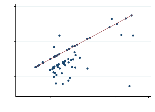
Figure 8: Measurement Error in FPDS Initial Entries

6 8 10 12 14 16

Log Contract Value: FPDS Initial Entry

8 10 12 14 16

Log Contract Value: Actual

Notes: Figure displays the (log) contract value according to the initial entry in the Federal Procurement Data

System (FPDS) versus the actual initial (log) contract value. The actual initial contract value was obtained for

a sample of 75 completed contracts from the analysis sample. Roughly three-quarters of the points lie below

the 45-degree line (plotted in red), which indicates systematic underreporting in the FPDS relative to the true

contract value. The initial measure from the FPDS corresponds to “Base And All Options Value”, which is the

largest of the three measures reported in each FPDS entry.

of the 75 contracts show underreporting in the initial entry in the FPDS. The median (mean)

difference is -1.099 log points, corresponding to a 67 percent difference.

Examining each of the 75 contracts shows that measurement error arises from a variety of

inconsistencies in how data are entered into FPDS. One error that occurs with some frequency

is that the user enters only the contract value for that ﬁscal year, rather than the full value of

the contract. In the sample of 75 contracts, the median duration is 3 years, so applying this

error across all the contracts would result underreporting of 67 percent as above. Because the

typical building cleaning contract is 3 to 4 times longer that the average service contract, this

error may be of more importance for this category relative to other service contracts; however,

other forms of entry error could also lead to systematic underreporting.

Another common entry error is that the user enters the amount of dollars obligated across

all three of the variables for contract value, rather than indicating the total value of the contract

using base and all options value. Table 16 provides an example of the ﬁrst ﬁve entries in FPDS

corresponding to a single contract. The entry for the total value is equivalent to the dollars

obligated in the ﬁrst entry ($10,740), as well as in all following entries. According to the posting

on FedBizOpps on January 26, 2010, the total value of the ﬁve-year contract (“Contract Award

Dollar Amount”) was $54,300. This is equal to the sum of dollars obligated across all 13 entries

in FPDS for the contract. The amounts entered in FPDS in these cases are best interpreted as

accounting measures for past and current payments, rather than future obligations that capture

Table 16: Entries in FPDS for an Example Contract

modnumber reasonformodiﬁcation effectivedate ultimatecompletiondate dollarsobligated baseandalloptionsvalue

0 1/1/2010 12/31/2014 10740 10740

1 C: FUNDING ONLY ACTION 12/8/2010 12/8/2010 2700 2700

2 M: OTHER ADMINISTRATIVE ACTION 4/14/2011 9/30/2011 900 900

3 C: FUNDING ONLY ACTION 5/6/2011 9/30/2011 4500 4500

4 C: FUNDING ONLY ACTION 10/18/2011 3/31/2012 5415 5415

... ... ... ... ... ...

Notes: Table displays the ﬁrst ﬁve entries in FPDS corresponding to contract PIID AG0276P100005. This contract

illustrates a typical entry mistake in FPDS, where the user enters the same amount for dollars obligated and the total

value of the contract (base and all options value). On the FedBizOpps website, a posting dated January 26, 2010

states the total value of the ﬁve-year contract (“Contract Award Dollar Amount”) of $54,300. The total of dollars

obligated across all 13 entries in FPDS is equal to this value.

total contract value.

D.2 Constructing Accurate Measures of Contract Value

Though the initial entry is not reliable for estimating the total contract value, additional mea-

sures can be obtained from the FPDS that perform well. For example, if the same value of

dollars obligated are reported in consecutive years, then that value likely represents the annual

price of the contract. In supplemental work, I detail the steps to cross-check the data and dif-

ferent candidate measures for price and duration. These comparisons result in the following

recommendations:

Duration The maximum observed date in the contract, minus the start date in the ﬁrst entry

within a contract.

Price The price is the value of obligated dollars if it is the same (or within 10 percent) in consecu-

tive years. If this is not observable, use the maximum value of the three (summed) measures

of dollar amounts for the total value of the contract. Divide this by the duration measure

above to obtain the price.

Any missing values of price or duration in the FedBizOpps data are imputed with the above

values constructed from FPDS. Researchers interested working with the FPDS data may contact

the author for additional details about the measurement error in the FPDS data and the accu-

racy of variables constructed under alternative assumptions. Though these measures are not

completely free from measurement error, the cross-validation exercise suggests that they are

centered on the true value, as opposed to being systematically underreported. These measures

are most applicable to ﬁxed-price contracts, where the ex post payments are not subject to the

same degree of uncertainty as, for example, cost-plus contracts.

Figure 9: Cost Overruns or Measurement Error?

(a) Total Obligated vs. Actual Contract Value

8 10 12 14 16

Log Total Obligated

8 10 12 14 16

Log Contract Value: Actual

(b) Total Obligated vs. FPDS Initial Value

6 8 10 12 14 16

Log Total Obligated

6 8 10 12 14 16

Log Contract Value: FPDS Initial Entry

Notes: Figure displays the (log) total payments on a contract (total obligated) vs. two different measures

of initial contract value. Total payments are calculated from summing up dollars obligated across entries

in the FPDS. Panel (a) compares total payments to the actual value obtained for a sample of 75 completed

contracts. Panel (b) compares total payments to the initial reported contract value in the FPDS for the same

sample. Points lying above the 45-degree line (plotted in red) correspond to inferred cost overruns. The

median implied overrun in panel (a) is 0. The median implied overrun in panel (b) is 0.242 log points, or 27

percent. The fact that many of the points (61 percent) lie above the 45-degree line in panel (b) arises from

the measurement error in the initial FPDS entry, which is captured in Figure 8.

D.3 Is There Evidence of Cost Overruns?

Examining the initial contract value from a sample of contracts provides further evidence that

ex post incentive concerns may not be ﬁrst-order for building cleaning services. One indicator

of ex post incentive problems is the presence of cost overruns, or payments above and beyond

the initially agreed-upon amount.

By calculating the total amount paid on an individual contract and comparing it to the total

amount, we can examine whether the buyer (the government) ends up paying more in cost

overruns. The sample of 75 contracts used to benchmark these ﬁgures all ﬁnished before the

end of the data, so the total amounts reﬂect the full time series of payments.

Figure 9 examines cost overruns by plotting the (log) total amount obligated on the contract

against measures of the initial value of the contract. The red 45-degree line indicates exact

correspondence between the initial value and the total payments. Panel (a) compares the total

payments to the actual initial value of the contract. The total payments follow the initial value

of the payments quite closely. A regression of (log) total obligated on (log) initial contract value

returns a coefﬁcient of 0.99. The median cost overrun in the sample, deﬁned as the difference

between the two logged values, is zero.

Panel (b) compares the total payments to the total value according to the initial entry in

FPDS. The median implied overrun is 0.242 log points, or 27 percent. The majority of points

(61 percent) lie above the 45-degree line, suggesting a substantial degree of cost overruns.

Likewise, the 75 percentile of implied overruns is 1.27 log points, compared to only 0.05 log

points when using the actual initial value in panel (a). The fact that this panel suggest cost

overruns is a direct result of measurement error in the initial entry in FPDS. The underreporting

showing in Figure 8 translates to implied cost overruns. Measurement error is further captured

by a regression of (log) total obligated on (log) contract value according to the initial entry in

FPDS. The coefﬁcient estimate is only 0.57, compared to 0.99 when a more accurate measure

of initial value is used.

Thus, a comparison of payments made to actual initial contract value demonstrates that cost

overruns are not a signiﬁcant concern for this product category (building cleaning services with

an annual price less than $1 million). This provides suggestive evidence that ex post incentive

concerns are not ﬁrst-order in this market.

E Identiﬁcation Proofs

E.1 Some Lemmas

To demonstrate the following proofs, it will be useful to ﬁrst introduce several lemmas.

Lemma 1. For symmetric auctions with independent private values, E[b

1:N

] = E[c

2:N

This is a standard result and can be obtained directly by taking the expectation given the

equilibrium bid function. I omit the proof here.

Lemma 2. min b

1:N

= E[c

1:(N−1)

] for the IPV model when the support of c is bounded from below

by c > −∞.

Proof. The equilibrium bid function is given by

β(c; N) = c +

∞

[1 − F (ξ)]

N−1

dξ

[1 − F (c)]

N−1

Then the minimum bid is

β(c; N) = c +

∞

[1 − F (ξ)]

N−1

dξ

[1 − F (c)]

N−1

= c +

∞

[1 − F (ξ)]

N−1

dξ

= c + ξ[1 − F (ξ)]

N−1

∞

ξ(N − 1)f(ξ)[1 − F (ξ)]

N−2

dξ

= c + (0 − c) +

∞

ξ(N − 1)f(ξ)[1 − F (ξ)]

N−2

dξ

= E[c

1:(N−1)

]

Where the third line comes from integration by parts. Here we require the assumption that

lim

ξ→∞

f(ξ)[1 − F (ξ)]

= 0, so that

ξ[1 − F (ξ)]

N−1

∞

= lim

γ→0

[1 − F (

)]

N−1

− c[1 − F (c)]

N−1

= lim

γ→0

−(N − 1)f(

)[1 − F (

)]

N−2

− c

= 0 − c

Lemma 3. The expected k-th order statistic of N draws can be written in terms of the expected

k-th and (k + 1) − th order statistics from N + 1 draws: E[c

k:N

] =

N+1

E[c

(k+1):(N +1)

] +

N+1−k

N+1

E[c

k:(N +1)

]

Proof. First, examining the difference between the k-th order statistics of N and N + 1 draws.

Expressing E[c

k:N

] − E[c

k:(N +1)

] and rearranging terms gives:

E[c

k:N

] − E[c

k:(N +1)

]

(k − 1)!(N − k)!

cf(c)F (c)

k−1

[1 − F (c)]

N −k

dc −

(N + 1)!

(k − 1)!(N + 1 − k)!

cf(c)F (c)

k−1

[1 − F (c)]

N +1−k



N!(N + 1 − k)

(k − 1)!(N + 1 − k)!

−

(N + 1)!

(k − 1)!(N + 1 − k)!

[1 − F (c)]



cf(c)F (c)

k−1

[1 − F (c)]

N −k

(N + 1)!

(k − 1)!(N + 1 − k)!

cf(c)F (c)

[1 − F (c)]

N −k

dc −

kN!

(k − 1)!(N + 1 − k)!

cf(c)F (c)

k−1

[1 − F (c)]

N −k

(N + 1 − k)



E[c

(k+1):(N +1)

] − E[c

k:N

]



Rearranging, we obtain

E[c

k:N

] =

N+1

E[c

(k+1):(N +1)

] +

N+1−k

N+1

E[c

k:(N +1)

E.2 Proof of Proposition 5

Consider the entry equation

E[π

· U · h(x)|n, T ] − k(m)· > 0 ⇐⇒ N ≥ n (20)

=⇒ E[π

|n, T ] ·

h(x)

k(m)

> ε ⇐⇒ N ≥ n (21)

For any realization (T, x, m), there exists (T, x

, m

) such that Pr(N ≥ n|T, x, m) = Pr(N ≥

n|T, x

, m

) for all N.

Using these values x

and m

that provide the same conditional distri-

bution of N, calculate:

E[B · U · h(x)|N, T, x, m]

E[B · U · h(x

)|N, t, x

, m

]

E[B|N, t] · E[U|N, T, x, m] · h(x)

E[B|N, t] · E[U|N, t, x

, m

] · h(x

)

h(x)

h(x

)

. (22)

As h(x) is normalized to 1 at x = x

, h(·) is identiﬁed.

Once h(·) is identiﬁed, E[B|N, T, x, m] is identiﬁed by calculating the mean of the scaled

(conditional) winning bid E[

h(x)

B · U · h(x)|N, T, x, m]. Recall that B · U · h(x) is the observed

winning bid.

k(·) is identiﬁed by the relation

h(x)

k(m)

h(x

)

k(m

)

(23)

based on the identiﬁcation of h(·) and the normalization k(m

) = 1 for an arbitrary m

Relative proﬁts are identiﬁed by considering different values of x and m that generate N

and N

6= N with the same probability. For every (N, T, x, m), there exists (N

, T, x

, m

) for

Here, and once more in the proof, I rely on either h(·) or k(·) having broad support.

which Pr(N ≥ n|T, x, m) = Pr(N

≥ n|T, x

, m

). Here, I re-use notation; x

and m

are

different from the ﬁrst part of this section. Thus, the entry condition

E[π

|N, T ] ·

h(x)

k(m)

= E[π

, t] ·

h(x

)

k(m

)

(24)

can be used to solve for

E[π

|N,T ]

E[π

,T ]

, as h(·) and k(·) are identiﬁed. Analogously, relative proﬁts

E[π

|N,T ]

E[π

|N,T

]

are identiﬁed.

It is straightforward to extend these identiﬁcation results to setting in which sellers observe

U prior to entry. This is possible because the distribution of U conditional on (T, x, m) will be

equal to the distribution of U conditional on (T, x

, m

E.3 Proof of Proposition 6

The ratio of expected proﬁts for n and n

conditional on T is given by

R =

E[π

|n, T ]

E[π

, T ]

(E[B|n, T ] − E[C|n, T ])

(E[B|n

, T ] − E[C|n

, T ])

(25)

As shown by Proposition 5, R is identiﬁed. Let n

= n + 1.

When the selection mechanism is a symmetric auction. E[B|n, T ] = E[C

2:n

|T ] and E[C|n, T ] =

E[C

1:n

|T ]. From here on I suppress notation indicating that costs are conditional on T . From

Lemma (3), we have E[C

1:n

] =

n+1

E[C

2:(n+1)

n+1

E[C

1:(n+1)

]. Plugging this into the equation

for R obtains



E[C

2:(n+1)

] − E[C

1:(n+1)

]



= E[C

2:n

] −

n + 1

E[C

2:(n+1)

] −

n + 1

E[C

1:(n+1)

]



R +

n + 1



E[C

1:(n+1)

] = E[C

2:n

] −



R +

n + 1



E[C

2:(n+1)

]

E[C

2:(n+1)

] and E[C

2:(n+1)

] are equivalent to E[B|N = n] and E[B|N = n + 1], both of

which are identiﬁed by Proposition 5. Therefore, E[C

1:(n+1)

] is identiﬁed. E[C

1:n

] is obtained

from equation (25). These are sufﬁcient to identify seller surplus.

Once seller surplus is identiﬁed, the distribution of ε is identiﬁed from equation (21) by

using variation in h(·) or k(·).

E.4 Proof of Proposition 7

For each observed sequential value of N ∈ {N, ..., N}, the ﬁrst-order and second-order statistics

of N draws from the cost distribution are identiﬁed (see Propositions 5 and 6). Using the

recursive relationship of order statistics shown in Lemma 3, these are equivalent to identifying

the ﬁrst N − N + 2 expected order statistics from N draws of C.

E.5 Alternative Identiﬁcation and a Note on Independent Private Values

The model in this paper allows for endogenous entry. To separate the private cost distribution

from unobservable heterogeneity, I make use of a entry cost shifter m to generate exogenous

variation in N. Without endogenous entry, there is no entry cost shifter and the entry equation

cannot be used to identify the model. When N is purely exogenous, variation in N can still be

used to separately identify the private and common cost distributions.

Proposition 10. First-price, symmetric auctions with unobserved heterogeneity and conditionally

independent private values are identiﬁed when only the winning bid and the number of bidders

is observed. In particular, seller surplus and the ﬁrst (N − N + 2) expected order statistics of N

draws from F are identiﬁed. Identiﬁcation is obtained without modeling entry as long as there is

no selection on unobservables.

The result can be generalized to auction settings that are independent of the duration-

setting problem. Thus, this identiﬁcation result may prove practical. With only the winning

bid and variation in the number of bidders, researchers can estimate a model with unobserved

heterogeneity, which is far less restrictive than the assumption of independent private values

(IPV) that is common in such settings with limited data.

This implies that in any setting where estimation is motivated by IPV, one could also es-

timate a conditional independent private values model with unobserved heterogeneity. The

econometrician may expect that unobserved heterogeneity is present, and this provides a theo-

retical background to test for its importance. In Appendix G, I detail a computational approach

that greatly speeds up the maximum likelihood estimation of these models.

Proof. The ratio of second-order statistics is identiﬁed by comparing winning bids B · U · h(x)

for different values of n and n

E[B|n, T, x, m] · E[U |n, T, x, m] · h(x)

E[B|n

, T, x, m] · E[U|n

, T, x, m] · h(x)

E[C

2:n

|T, x, m]

E[C

2:n

|T, x, m]

(26)

where E[U|n, T, x, m] = E[U|n

, T, x, m] = E[U|T, x, m] by independence and no selection on

unobservables.

From here on, C

and U may be conditional on (T, x, m). I suppress this in my notation for

clarity. Normalizing E[U ] = 1 pins down the scale of E[C

2:n

Suppose that another (

F ,

G) rationalizes the data. Then

· U

Note that, in practice, we may normalize E[U|T, x, m] = 1 for all (T, x, m) realizations. How the mean of

2:n

· U changes is captures in changes to the mean of C.

Construct

U, and

U as random variables that are independent of and have the same

conditional distributions as their tilde-free counterparts. Then it follows that

· U) ·













=⇒ B

From this relation, we may take the minimum on both sides. By independence and Lemma

2, I obtain

E[C

1:(n−1)

] · E[

1:(n

−1)

] = E[

1:(n−1)

] · E[C

1:(n

−1)

]

E[C

1:(n−1)

]

E[C

1:(n

−1)

]

1:(n−1)

]

1:(n

−1)

]

That is, any (

F ,

G) that rationalizes the data has a private cost distribution with the same

ratio of ﬁrst order statistics.

Finally, using the fact that E[C

1:(n−1)

] =

E[C

2:n

] +

n−1

E[C

1:n

], we can link together these

ratios when n

= n + 1.

E[C

2:n

] +

n−1

E[C

1:n

]

E[C

1:n

]

2:n

] +

n−1

1:n

]

1:n

]

=⇒

E[C

2:n

]

E[C

1:n

]

2:n

]

1:n

]

As we have identiﬁed E[C

2:n

], E[C

1:n

] and E[C

1:(n−1)

] is also identiﬁed. Therefore,

F and

F have the same ratio of second-order statistics. With sequential values of N ∈ {N , ..., N }, we

can iterate forward from the from the identiﬁed ﬁrst-order and second-order statistics using the

recursive relationship between order statistics from Lemma 3. Therefore,

F and F and identical

up to the ﬁrst N − N + 2 expected order statistics from N draws of C.

F A Model with Microfoundations

In the empirical application of this paper, I employ a “reduced-form” approach to a capturing

how the distribution of private costs changes with T. Here, I provide a model of underlying costs

that generates both the distribution of costs and how duration affects the distribution. Suppose

that instantaneous costs follow an Ornstein-Uhlenbeck diffusion process. The continuous-time

cost process X

is governed by the differential equation

= θ(µ − x

) + γdW

where W

is a Wiener process. This process is stationary over t. That is, any contract with

duration T will have the same unconditional distribution as any other contract with duration

T . Deﬁne the average cost over time T as

Then c

is Gaussian with mean µ and variance σ



θT + e

−θT

− 1



. When costs are

Gaussian, E[c

1:N

(σ)] = E[z

1:N

]σ + µ, where z is a standard normal.

First, consider the efﬁcient contract. Let ξ(T ) = σ =

(θT + e

−θT

− 1). For ease of

exposition, assume β = 1. The efﬁcient contract T solves

min

E[z

1:N

]ξ(T ) + µ +

As E[z

1:N

] is negative and the variance of c

is decreasing with T , the average expected

supply cost µ + E[z

1:N

]ξ(T ) is increasing with T . In this microfounded model, the increasing

supply costs over many periods is due the idiosyncratic variation over time. The mean expected

supply cost for each bidder, µ, is constant over time.

Likewise, the same analysis applies to the buyer-optimal contract when N > 3. The buyer

solves the same problem where the second-order statistic E[z

2:N

] is substituted for E[z

1:N

]. For

N ∈ {2, 3}, E[z

2:N

] > 0.

F.1 Relating Competition to Contract Duration

The ﬁrst-order condition from the problem above is

E[z

1:N

]ξ

(T ) =

−ξ

(T )T

= −

E[z

1:N

]

. (27)

In this case, we obtain a monotonic relationship between the number of bidders and the

optimal duration, as N has a monotonic effect on the right-hand side. Unlike the U-shape

models, the microfounded model here does not have a lower bound on costs.

Proposition 11. The efﬁcient duration is decreasing in the number of bidders.

Proof.



−ξ

(T )T



= −2T · ξ

(T ) − T

(T ). Combining the second-order conditions and

ﬁrst-order conditions, we obtain.

E[z

1:N

]ξ

(T ) > −

E[z

1:N

]ξ

(T )

=⇒ T

· ξ

(T ) < −2Tξ

(T )

An increase in N increases the RHS of equation 27. As



−ξ

(T )T



< 0, the optimal T

falls.

We now turn to the buyer-optimal contract, which solves the same problem where the

second-order statistic E[z

2:N

] is substituted for E[z

1:N

Proposition 12. The buyer-optimal duration is decreasing in the number of bidders. It is optimal

for the buyer to issue a permanent contract for N ∈ {2, 3}.

The permanent contract result follows from the fact that the second-order statistic is greater

than zero with a small N.

Additionally, we have that E[z

1:N

] < E[z

2:N

]. Therefore,

Proposition 13. The efﬁcient duration is less than the buyer-optimal duration.

G Likelihood Function

For estimation, we obtain the likelihoods for Y

and N given by

|N,X,T,M

|T,N

(

h(x)

)

h(x)

U|N,T,x,m

(U)dU

Pr(N = n|T, x, m) =

Pr(N = n|U, T, x, m)f

U|T,x,m

(U)dU

For estimation, I make the assumption that U ⊥⊥ (X, M). As U is not observed by the buyer

when setting T , U ⊥⊥ (T, x, m). This simpliﬁes the problem so that f

U|T,x,m

(U) = f

(U).

The conditional distribution of U used in the likelihood of Y

is given by f

U|N,T,x,m

(u) =

Pr(N=n|U,T,x,m)f

(u)

Pr(N=n|T,x,m)

. This simpliﬁes so that the joint contribution is given by

|N,X,T,M

) · Pr(N = n|T, x, m) =



|T,N

(

h(x)

)

h(x)

U|N,T,x,m

(u)du



Pr(N = n|T, x, m)



|T,N

(

h(x)

)

h(x)

Pr(N = n|u, T, x, m)f

(u)

Pr(N = n|T, x, m)



Pr(N = n|T, x, m)

|T,N

(

h(x)

)

h(x)

Pr(N = n|u, T, x, m)f

(u)du

With the assumption that the shock ε is independent of (U, T, x, m), we have the following

expression for conditional probability of N.

Pr(N = n|U, T, x, m) = F

ln ε

(ln E[π

|T ] + ln h(x) + ln U − ln k(m))

−F

ln ε

(ln E[π

n+1

|T ] + ln h(x) + ln U − ln k(m))

I use the joint likelihood of Y

and N to obtain estimates for cost and entry parameters.

G.1 A Computational Innovation

In this setting, there is a symmetric equilibrium in which each bidder has a monotone bid

function β(·; n) mapping private costs to the submitted bid. The density of an observed bid is

given by

(b; n) = f

(β

−1

(b; n))

(β

−1

(b; n))

In maximum likelihood estimation of the cost distribution, it is necessary to invert the bid

function to calculate the density. This can be computationally intensive when β does not have

a closed-form solution.

In the presence of unobserved heterogeneity, the density of the observed bid

B = B · U is

given by the convolution when B ⊥⊥ U.

(

b) =

(u)du

−1

; n



−1



; n



(u)du

Here, the computational burden increases greatly. Integrating out the unobserved hetero-

geneity means that the bid function must be inverted for each value of u within the integral in

order to calculate β

−1



; n



. As the inverse bid function has an analytic solution for only a

few specialized cases, in practice this computation relies on a non-linear equation solver or an

approximation. Thus, the calculations are constrained by the efﬁciency and accuracy of such

an approach.

One easy-to-implement solution that makes maximum likelihood signiﬁcantly more tractable

is to use a change-of-variables to calculate the density. Instead of integrating out the unobserved

heterogeneity by integrating over u, replace u with u =

β(c)

and integrate over c. The density

then becomes:

(

b) =

−1



−1





(u)du

−1

(u)

−1

(u)



−1

(β(c))



(β

−1

(β(c)))

β(c)

−

β(c)

(c)

β(c)

Note that in this form, there is no need to invert the bid function. As the general form for

the symmetric equilibrium bid function is

β(c) = c +

∞

[1 − F (z)]

n−1

[1 − F (c)]

n−1

the primary computational cost is a numerical integration routine. Therefore, the model is

computationally tractable for a vast class of parametric distributions of C and U , as well as

nonparametric approximations such as B-splines. This innovation can also apply to models

with additively separable unobserved heterogeneity as well. When

B = B + U, then

(

b) =



−1



b − u



(u)du =



b − β(c)





−β

(c)



dc.

H Supplemental Empirical Results

H.1 Distributions of Bidder Costs

Figure 10: Distribution of Bidder Costs

(a) Duration-Dependent Private Costs

0.00

0.03

0.06

0.09

0 10 20 30 40

Private Costs (Annual)

Density

Duration

(b) Unobservable Auction-Speciﬁc Heterogeneity

0.00

0.25

0.50

0.75

0 1 2 3

Multiplicative Unobserved Auction−Specific Costs

Density

Notes: The ﬁgure plots the distributions of the unobservable components of bidder costs.

Private costs are displayed in panel (a), and the density of unobserved auction-speciﬁc

heterogeneity is displayed in panel (b). In panel (a), the density is plotted for a one-

year contract and a ﬁve-year contract. The estimated parameters indicate an increasing

mean and a decreasing variance in private costs with contract duration. The density shifts

smoothly between these functions for intermediate values of duration.

H.2 Projecting Transaction Costs on Location Type and Agency

Table 17: Dependent Variable: ln(Transaction Costs)

(1) (2)

Location Type: Accommodations 1.436

∗∗∗

(0.278) 0.249 (0.219)

Location Type: Airport 0.414 (0.264) 0.543

∗∗∗

(0.203)

Location Type: Field Ofﬁce 0.027 (0.125) 0.068 (0.095)

Location Type: Industrial 1.150

∗∗∗

(0.325) 0.331 (0.254)

Location Type: Medical 1.530

∗∗∗

(0.256) 0.294 (0.201)

Location Type: Ofﬁce 0.000 (.) 0.000 (.)

Location Type: Research 0.371

∗∗

(0.157) 0.232

∗

(0.120)

Location Type: Services 0.180 (0.207) 0.005 (0.158)

Location Type: Technical 1.403

∗∗∗

(0.272) 0.285 (0.212)

Location Type: Visitors 0.784

∗∗∗

(0.196) 0.319

∗∗

(0.152)

Department: Agriculture 0.309

∗∗

(0.123) −0.183

∗

(0.096)

Department: Commerce 0.559

∗∗∗

(0.177) 0.292

∗∗

(0.137)

Department: Defense 0.000 (.) 0.000 (.)

Department: GSA 1.577

∗∗∗

(0.240) 0.418

∗∗

(0.189)

Department: Homeland Security 1.645

∗∗∗

(0.217) 0.650

∗∗∗

(0.171)

Department: Interior 0.440

∗∗

(0.193) −0.095 (0.149)

Department: Other 1.071

∗∗∗

(0.252) 0.256 (0.195)

Department: Veterans Affairs 0.177 (0.235) 0.404

∗∗

(0.180)

ln(Square Footage) 0.601

∗∗∗

(0.026)

ln(Weekly Frequency) 0.431

∗∗∗

(0.059)

Standard errors in parentheses

∗

p < 0.10,

∗∗

p < 0.05,

∗∗∗

p < 0.01

Notes: The table displays results for regressions of estimated (log) transaction costs on location

type and department, with additional controls in speciﬁcation (2). N =1,046.

H.3 Incumbency and Asymmetries

In this section, I present regressions for the dependent variables of price and the number of

bids, including an indicator for whether or not a single incumbent bidder was identiﬁed from

a previous contract. That is, the indicator equals one if building cleaning services for the same

agency and 9-digit ZIP code were performed by a single supplier in the previous year. The

coefﬁcient on this variable is not signiﬁcant, and its inclusion does not meaningfully impact the

estimated coefﬁcients.

Table 18: Descriptive Regressions: Incumbency Check, Price

IV-1 (a) IV-1 (b) IV-1 (c) IV-2 (a) IV-2 (b) IV-2 (c)

Number of Bids −0.053

∗∗

−0.052

∗∗

−0.052

∗∗

−0.047

∗∗

−0.046

∗∗

−0.046

∗∗

(0.022) (0.022) (0.022) (0.022) (0.022) (0.022)

Duration (Years) 0.043

∗∗∗

0.043

∗∗∗

0.043

∗∗∗

0.033

∗∗

0.033

∗∗

0.033

∗∗

(0.016) (0.016) (0.016) (0.015) (0.015) (0.015)

ln(Square Footage) 0.689

∗∗∗

0.688

∗∗∗

0.688

∗∗∗

0.687

∗∗∗

0.686

∗∗∗

0.686

∗∗∗

(0.024) (0.024) (0.024) (0.024) (0.024) (0.024)

ln(Weekly Frequency) 0.467

∗∗∗

0.467

∗∗∗

0.467

∗∗∗

0.407

∗∗∗

0.407

∗∗∗

0.407

∗∗∗

(0.041) (0.041) (0.041) (0.040) (0.040) (0.040)

ln(2004 Unemp.) 0.080

∗∗∗

0.080

∗∗∗

0.080

∗∗∗

0.060

∗∗∗

0.060

∗∗∗

0.060

∗∗∗

(0.019) (0.019) (0.019) (0.018) (0.018) (0.018)

High-Intensity Cleaning 0.559

∗∗∗

0.559

∗∗∗

0.559

∗∗∗

−0.076 −0.076 −0.077

(0.075) (0.075) (0.075) (0.125) (0.125) (0.125)

Follow-On Contract 0.018 −0.003

(0.053) (0.050)

Incumbent Winner 0.012 −0.008

(0.106) (0.100)

Site Type FEs X X X

Observations 1046 1046 1046 1046 1046 1046

0.69 0.69 0.69 0.73 0.73 0.73

Standard errors in parentheses

∗

p < 0.10,

∗∗

p < 0.05,

∗∗∗

p < 0.01

Notes: The table displays regression results for regressions of log annual price on auction characteristics and

local market characteristics. Speciﬁcations IV-1 (a) and IV-2 (a) are two-stage least squares regressions and

are identical to the descriptive regressions in Table 2. The (b) speciﬁcations include an additional regressor

indicating whether the contract is a follow-on contract and the (c) speciﬁcations include an indicator for

whether the contract was won by an incumbent bidder in a follow-on contract.

Table 19: Descriptive Regressions: Incumbency Check, Number of Bids

(1) (2) (3) (4) (5) (6)

Duration (Years) −0.002 −0.005 −0.009 −0.002 −0.005 −0.009

(0.099) (0.099) (0.099) (0.100) (0.100) (0.100)

ln(Square Footage) 0.834

∗∗∗

0.835

∗∗∗

0.840

∗∗∗

0.825

∗∗∗

0.824

∗∗∗

0.829

∗∗∗

(0.106) (0.106) (0.106) (0.112) (0.112) (0.112)

ln(Weekly Frequency) 0.009 0.014 0.010 0.137 0.146 0.141

(0.253) (0.253) (0.253) (0.257) (0.258) (0.257)

ln(2004 Unemp.) −0.794

∗∗∗

−0.809

∗∗∗

−0.813

∗∗∗

−0.793

∗∗∗

−0.808

∗∗∗

−0.811

∗∗∗

(0.238) (0.239) (0.239) (0.238) (0.238) (0.238)

ln(Unemployment) 1.420

∗∗∗

1.432

∗∗∗

1.436

∗∗∗

1.356

∗∗∗

1.366

∗∗∗

1.370

∗∗∗

(0.231) (0.231) (0.231) (0.231) (0.231) (0.231)

ln(Num. Firms in Zip3) 0.257

∗

0.248

∗

0.250

∗

0.276

∗

0.267

∗

0.269

∗

(0.148) (0.148) (0.148) (0.147) (0.147) (0.147)

Generic Set-Aside 1.134

∗∗∗

1.125

∗∗∗

1.131

∗∗∗

0.987

∗∗∗

0.982

∗∗∗

0.985

∗∗∗

(0.350) (0.350) (0.350) (0.361) (0.361) (0.361)

High-Intensity Cleaning −0.294 −0.303 −0.305

(0.475) (0.475) (0.475)

Follow-On Contract −0.351 −0.353

(0.326) (0.326)

Incumbent Winner −0.836 −0.814

(0.650) (0.646)

Site Type FEs X X X

Observations 1046 1046 1046 1046 1046 1046

0.17 0.17 0.17 0.19 0.19 0.19

Standard errors in parentheses

∗

p < 0.10,

∗∗

p < 0.05,

∗∗∗

p < 0.01

Notes: The table displays regression results for regressions of number of bids on auction characteristics and

local labor market variables. Speciﬁcations (1) and (4) are equivalent to the descriptive regressions (3) and

(4) in Table 3. The additional speciﬁcations included indicators for whether the contract is a follow-on contract

or whether the contract was won by an incumbent bidder in a follow-on contract.

H.4 Detailed Impacts of Standardized Duration

Table 20: Percent Impact of Uniform Term Policies

T Affected Price Trans. Cost Total Cost Count

1 All −11.2 317.1 33.7 1046

T >

T −11.8 334.2 35.5 995

T <

T 1.5 −36.6 0.6 23

2 All −7.5 108.5 9.0 1046

T >

T −8.7 125.4 10.0 930

T <

T 4.1 −50.5 2.3 62

3 All −3.9 39.0 2.9 1046

T >

T −6.3 61.8 3.4 761

T <

T 5.1 −42.6 2.7 146

4 All −0.4 4.3 1.3 1046

T >

T −3.2 24.0 0.7 686

T <

T 6.0 −39.1 2.9 306

5 All 3.1 −16.6 1.5 1046

T >

T −2.0 12.2 0.3 18

T <

T 6.9 −36.8 3.3 478

Notes: The table displays the average percent changes (by contract, not in aggre-

gate) in total costs, prices, and annualized transaction costs when all contracts

are issued in standardized durations corresponding to

T . For a uniform duration

policy of 4 years or less, the average price paid decreases and the amount spent

on transaction costs increases. The ﬁnal column lists the count of the affected

contracts. The ﬁrst column indicates the group affected by the policy. Rows cor-

responding to T >

T pertain to all contracts that see a reduction in duration, and

the reported effects are equivalent to a policy that caps duration at

T .