Unemployment Insurance and Job Search in the Great Recession

143

JESSE ROTHSTEIN

University of California, Berkeley

Unemployment Insurance and

Job Search in the Great Recession

ABSTRACT More than 2 years after the ofﬁcial end of the Great Reces-

sion, the labor market remains historically weak. One candidate explanation

is supply-side effects driven by dramatic expansions of unemployment insur-

ance (UI) beneﬁt durations, to as long as 99 weeks. This paper investigates

the effect of these extensions on job search and reemployment. I use the lon-

gitudinal structure of the Current Population Survey to construct unemploy-

ment exit hazards that vary across states, over time, and between individuals

with differing unemployment durations. I then use these hazards to explore

a variety of comparisons intended to distinguish the effects of UI extensions

from other determinants of employment outcomes. The various speciﬁcations

yield quite similar results. UI extensions had signiﬁcant but small negative

effects on the probability that the eligible unemployed would exit unemploy-

ment. These effects are concentrated among the long-term unemployed. The

estimates imply that UI extensions raised the unemployment rate in early 2011

by only about 0.1 to 0.5 percentage point, much less than implied by previous

analyses, with at least half of this effect attributable to reduced labor force exit

among the unemployed rather than to the changes in reemployment rates that

are of greater policy concern.

lthough the so-called Great Recession ofﬁcially ended in June 2009,

the labor market remains stagnant. In November 2011 the unemploy-

ment rate was 8.6 percent, only the third time in 2.5 years that it was below

9 percent. Nearly 45 percent of the unemployed had been out of work for

more than 6 months.

An important part of the policy response to the Great Recession has been

a dramatic expansion of unemployment insurance (UI) beneﬁts. Preexist-

ing law provided for up to 26 weeks of beneﬁts, plus up to 20 additional

weeks under the Extended Beneﬁts (EB) program in states experiencing

high unemployment rates. But in past recessions Congress has frequently

144 Brookings Papers on Economic Activity, Fall 2011

authorized additional weeks on an ad hoc basis, and in June 2008 it enacted

the Emergency Unemployment Compensation (EUC) program, which, in

a series of extensions, has brought statutory beneﬁt durations to as long as

99 weeks.

Unemployment beneﬁts subsidize continued unemployment. Thus, it

seems likely that the unprecedented UI extensions have contributed to

some degree to the elevated unemployment rate. However, the magnitude

and interpretation of this effect are not clear. Several recent analyses have

found that the extensions contributed around 1.0 percentage point to the

unemployment rate in 2010 and early 2011 (see, for example, Mazumder

2011, Valletta and Kuang 2010, Fujita 2011), and some observers have

claimed that the effects were several times that size.

There are two channels by which UI can raise unemployment, with very

different policy implications (Solon 1979). On the one hand, UI beneﬁts

can lead recipients to reduce their search effort and raise their reservation

wage, slowing the transition into employment. On the other hand, these

beneﬁts, which are available only to those engaged in active job search,

provide an incentive for continued search for those who might otherwise

exit the labor force. This second channel raises measured unemployment

but does not reduce the reemployment of displaced workers. Partly on the

basis of this observation, David Howell and Bert Azizoglu (2011) ﬁnd “no

support” for the view that the recent UI extensions reduced employment.

Unfortunately, most studies of the effect of UI on the duration of unem-

ployment have been unable to distinguish the two channels.

Determining the portion of any rise in unemployment attributable to UI

extensions on labor market outcomes is difﬁcult because these extensions

are endogenous by design. UI beneﬁts are extended in severe recessions

precisely because it is seen as unreasonable to demand that workers ﬁnd

jobs quickly when the labor market is weak. Thus, obtaining a credible

estimate of the effect of the recent UI extensions requires a strategy for

distinguishing this effect from the confounding inﬂuence of historically

weak labor demand.

This paper uses the haphazard rollout of the EUC and EB programs dur-

ing the Great Recession and its aftermath to identify the partial equilibrium

effects of the recent UI extensions on the labor market outcomes of work-

ers who have lost their jobs and are actively seeking new employment.

I use the longitudinal structure of the Current Population Survey (CPS) to

1. Grubb (2011); Robert Barro, “The Folly of Subsidizing Unemployment,” Wall Street

Journal, August 30, 2010.

JESSE ROTHSTEIN 145

2. In addition, UI may reduce hysteresis by increasing labor force attachment and

thereby slowing the deterioration of job skills. If so, UI extensions could make displaced

workers more employable when demand recovers. A related possibility is that UI extensions

deter displaced workers from claiming disability payments (Duggan and Imberman 2009,

Joint Economic Committee 2010).

construct hazard rates for unemployment exit, reemployment, and labor

force exit that vary across states, over time, and between individuals enter-

ing unemployment at different dates.

I explore a variety of strategies for isolating the effects of UI exten-

sions. One strategy exploits the gradual rollout and repeated expiration of

EUC beneﬁts through successive federal legislation to generate variation

in beneﬁt durations across labor markets facing plausibly similar demand

conditions. Second, following a recent study by Rob Valletta and Kath-

erine Kuang (2010), I use UI-ineligible job seekers as a control group for

eligible unemployed workers in the same state and month. A third strategy

exploits decisions by individual states to take up or decline optional EB

provisions that alter the availability of beneﬁts; this strategy uses a “con-

trol function” to distinguish the effects of the economic conditions that

deﬁne eligibility. Finally, I exploit differences in remaining beneﬁt eligibil-

ity among UI-eligible workers displaced at different times, but searching

for work in the same labor markets, to identify the effect of approaching

beneﬁt exhaustion.

All of the strategies point to broadly similar conclusions. The availabil-

ity of extended UI beneﬁts (under both EB and EUC) caused small reduc-

tions in the probability that an unemployed worker exited unemployment,

reducing the monthly hazard in the fourth quarter of 2010, when the aver-

age unemployed worker anticipated a total beneﬁt duration of 65 weeks, by

between 1 and 3 percentage points on a base of 22.4 percent. Not more than

half of this unemployment exit effect comes from effects on reemployment:

my preferred speciﬁcation indicates that UI extensions reduced the average

monthly reemployment hazard of unemployed job losers in 2010Q4 by

0.5 percentage point (on a base of 13.4 percent) and reduced the monthly

labor force exit hazard by 1.0 percentage point (on a base of 9.0 percent).

The labor force exit effect raises the possibility that UI extensions

actually raise the reemployment rate of those who lose their jobs in bad

economic times, by extending the time until they abandon their search.

However, estimating this effect requires strong assumptions, along with

ad hoc corrections for shortcomings in the data. Using such assumptions

and corrections, I simulate the effect of the 2008–10 UI extensions on

aggregate unemployment and on the fraction of unemployed workers out of

146 Brookings Papers on Economic Activity, Fall 2011

work 27 weeks or more (the long-term unemployment share). All of the esti-

mates are of partial equilibrium effects, as I ignore any effects of reduced

job search by one worker on others’ search behavior or job ﬁnding rates.

This almost certainly leads me to overstate the effect of UI extensions.

Nevertheless, I ﬁnd quite small effects. My preferred speciﬁcation

indicates that in the absence of UI extensions, the unemployment rate in

December 2010 would have been about 0.2 percentage point lower, and

the long-term unemployment share would have been about 1.6 percentage

points lower. Even the speciﬁcation yielding the largest effects indicates

that UI extensions contributed only 0.5 percentage point to the unemploy-

ment rate. Moreover, simulations that include only the labor force partici-

pation effects yield estimates at least half as large as do simulations with

both participation and reemployment effects, suggesting that reduced job

search due to UI extensions raised the unemployment rate by only 0.1 to

0.2 percentage point.

The remainder of the paper is organized as follows. Section I reviews

recent labor market trends and discusses the UI extensions that have been

an important part of the policy response. It also presents a simple model

of the effects of UI beneﬁt durations and reviews existing estimates of

the effect of the recent extensions. Section II discusses the longitudi-

nally linked CPS data that I use to study the effects of the UI extensions.

Section III presents my empirical strategies for isolating these effects.

Section IV reports estimates of the effect of UI beneﬁt durations on the

unemployment exit hazard. Section V develops a simulation methodol-

ogy that I use to extrapolate these estimates to obtain effects on labor

market aggregates, and presents results. Section VI concludes.

I. The Labor Market and Unemployment Insurance

in the Great Recession

The Great Recession ofﬁcially began in December 2007, but the downturn

was slow at ﬁrst: seasonally adjusted real GDP fell at an annual rate of only

1.8 percent in the ﬁrst quarter of 2008, then grew at a 1.3 percent rate in the

second quarter. Conditions then worsened sharply, and GDP contracted at

an annual rate of 8.9 percent in the fourth quarter of 2008.

I.A. Labor Market Trends

The labor market downturn also began slowly. Figure 1 shows that

the unemployment rate began trending up in 2007, but it remained only

5.8 percent as of July 2008. Over the next year, however, it rose 3.7 per-

JESSE ROTHSTEIN 147

centage points, to 9.5 percent, and it has fallen below 9 percent in only

three months since. Employment data show similar trends: nonfarm payroll

employment rose through most of 2007, fell by 738,000 in the ﬁrst half

of 2008, and then fell by nearly 6.8 million over the next 12 months. Job

losses continued at slower rates in the second half of 2009, followed by

modest and inconsistent growth in 2010. As of August 2011, employment

remained 6.9 million below its prerecession peak.

Figure 1 also shows the long-term unemployment share. This measure

has lagged the overall unemployment rate by about 6 months or perhaps a

bit more: it began to increase slowly in early 2008 and much more quickly

in late 2008, reaching a peak of around 45 percent in early 2010—nearly

20 percentage points higher than the previous record of 26.0 percent,

recorded in June 1983—and remaining mostly stable since then.

Figure 2 illustrates gross labor market ﬂows during and after the reces-

sion. These are obtained from two sources: the Job Openings and Labor

Turnover Survey (JOLTS), which derives from employer reports, and the

Long-term unemployment share

(right scale)

Unemployment rate

(left scale)

Percent Percent

2004 2005 2006 2007 2008 2009 2010 2011

Source: Bureau of Labor Statistics data.

a. Both series are seasonally adjusted monthly data.

b. Fraction of the unemployed who have been out of work 27 weeks or longer.

Figure 1. Unemployment and Long-Term Unemployment, 2004–11

148 Brookings Papers on Economic Activity, Fall 2011

2004 2005 2006 2007 2008 2009 2010 2011

2005 2006 2007 2008 2009 2010

2004 2011

2.5

2.0

1.5

1.0

0.5

3.0

2.5

2.0

1.5

1.0

0.5

Source: Bureau of Labor Statistics data.

a. All series are seasonally adjusted monthly data, smoothed with a 3-month symmetric triangular

moving average, y

= (y

t–1

+ 2y

+ y

t+1

)/4.

b. From the Job Openings and Labor Turnover Survey data, which derive from employer surveys.

c. From the research series on labor force status flows constructed by the BLS from longitudinally

linked monthly CPS files.

Millions

Millions Percent of previous month’s unemployed

Flows out of jobs

Flows into jobs and out of unemployment

Quits

Layoffs and discharges

E-U flows

Hires

(left scale)

U-E flow rate

(right scale)

U-N flow rate

(right scale)

Figure 2. Gross Labor Market Flows, 2004–11

JESSE ROTHSTEIN 149

3. See Elsby, Hobijn, and ¸S ahin (2010) for a more detailed examination of these and

other aggregate data.

gross ﬂows research series computed by the Bureau of Labor Statistics (BLS)

from matched monthly CPS household data, discussed at length below.

The top panel shows ﬂows out of work: quits and layoffs from the JOLTS

(“other separations,” including retirements, are not shown), and gross ﬂows

from employment to unemployment (E-U) from the CPS. The bottom

panel shows ﬂows into work: hires from the JOLTS and unemployment-

to-employment (U-E) ﬂows from the CPS. It also shows unemployment-

to-nonparticipation (U-N) ﬂows; both the U-E and the U-N ﬂows are

expressed as shares of the previous month’s unemployed population.

The two panels of ﬁgure 2 shed a good deal of light on the dynamics

of the rise and stagnation of the unemployment rate.

The top panel shows

that layoffs spiked and quits collapsed in late 2008, indicating an extreme

weakening of labor demand; interestingly, the decline in quits seems to

have preceded the increase in layoffs by several months. Not surprisingly,

the number of monthly E-U transitions increased by about one-third over

the course of 2008. Layoffs returned to (or even below) normal levels in

late 2009, but quits remained just over half of their prerecession level and

E-U ﬂows remained high, suggesting that weak demand continued to dis-

suade workers from leaving their jobs and to impede the usual quick transi-

tion of laid-off workers into new jobs.

The bottom panel of ﬁgure 2 shows that the collapse in new hires was

more gradual than the spike in layoffs and began much earlier, in late 2007.

The rate at which unemployed workers transitioned into employment also

began to decline at this time, then fell much more sharply in late 2008.

Recall that the rapid run-up in long-term unemployment was in mid-2009,

roughly 6 months later, again suggesting that the usual process by which

job losers are recycled into new jobs was substantially disrupted around

the time of the ﬁnancial crisis. U-E ﬂows remain very low at this writ-

ing. Finally, the U-N ﬂow rate fell rather than rose during the recession,

despite weak labor demand that might plausibly have led unemployed

workers to become discouraged. This is plausibly a consequence of UI

beneﬁt extensions, which created incentives for ongoing search even if the

prospect of ﬁnding a job was remote.

I.B. The Policy Response

Congress responded quickly to the deteriorating labor market, autho-

rizing the EUC program in June 2008, but proceeded in ﬁts and starts

150 Brookings Papers on Economic Activity, Fall 2011

4. This discussion draws heavily on Fujita (2010). I neglect a number of details of the UI

program rules. In particular, claimants whose tenure in their previous job was short are not

eligible for the full 26 weeks of regular beneﬁts.

thereafter.

The June 2008 legislation made 13 weeks of EUC beneﬁts

available to anyone who exhausted regular beneﬁts before March 28,

2009. The program was subsequently expanded in November 2008. That

expansion extended the original EUC (now called EUC tier I) beneﬁts to

20 weeks and added a second tier of 13 weeks of beneﬁts in states with

unemployment rates above 6 percent. A second expansion in November

2009 changed tier II beneﬁts to 14 weeks and added tier III, 13 weeks of

beneﬁts in states with unemployment rates above 6 percent, and tier IV,

an additional 6 weeks in states with unemployment rates above 8.5 per-

cent. Individuals in states qualifying for all four tiers were thus eligible for

53 weeks of EUC beneﬁts. The ﬁrst four columns of table 1 show the num-

ber of tiers and number of weeks available over time.

The EUC program was originally set to expire on March 28, 2009. How-

ever, the program was reauthorized several times to delay the scheduled

Table 1. Changes in the Emergency Unemployment Compensation Program over

2008–10

Weeks of beneﬁts available under EUC tier

Scheduled EUC

expirationDate

I II III

Jun. 30, 2008 13 Mar. 28, 2009

Nov. 21, 2008 20 13

Mar. 28, 2009

Feb. 17, 2009 20 13

Dec. 26, 2009

Nov. 6, 2009 20 14 13 6 Dec. 26, 2009

Dec. 19, 2009 20 14 13 6 Feb. 28, 2010

Feb. 28, 2010 0 0 0 0 NA

Mar. 2, 2010 20 14 13 6 Apr. 5, 2010

Apr. 5, 2010 0 0 0 0 NA

Apr. 15, 2010 20 14 13 6 Jun. 2, 2010

Jun. 2, 2010 0 0 0 0 NA

Jul. 22, 2010 20 14 13 6 Nov. 30, 2010

Nov. 30, 2010 0 0 0 0 NA

Dec. 17, 2010 20 14 13 6 Jan. 3, 2012

Dec. 23, 2011 20 14 13 6 Mar. 6, 2012

Source: Fujita (2010) and Department of Labor bulletins.

a. Dates on which legislation creating, changing, or reauthorizing the program was enacted or the

program expired. After each expiration, the eventual reauthorization was retroactive. NA = not applicable.

b. Beneﬁts available only in states with unemployment rates above 6 percent.

c. Beneﬁts available only in states with unemployment rates above 8.5 percent.

d. As this volume goes to press.

JESSE ROTHSTEIN 151

5. The Recovery Act also provided for tax deductibility of a portion of UI beneﬁts, for

somewhat expanded eligibility, and for more generous weekly beneﬁt amounts.

6. During the period covered by my sample, the minimal triggers provided beneﬁts only

when the 13-week moving average of the insured unemployment rate (IUR) was at least

5 percent and above 120 percent of the maximum of its values 1 year and 2 years earlier. It

is this lookback period that accounts for the decline in the minimal series in late 2009. The

maximal triggers also provided beneﬁts in states with 13-week IURs above 6 percent (regard-

less of their lagged values) or with a 3-month moving average total unemployment rate (the

traditional measure) above 6.5 percent and above 110 percent of the value either 1 or 2 years

earlier. Each simulated beneﬁts series allows a state’s status to change no more than once in

13 weeks, following program rules; the maximal series also assumes that the optional 3-year

lookback was adopted when it became available in 2011. See National Employment Law

Project (2011) and the Federal-State Extended Unemployment Compensation Act of 1970

(workforcesecurity.doleta.gov/unemploy/EB_law_for_web.pdf, accessed June 28, 2011).

expiration. The last column of table 1 shows the scheduled expiration date

as it changed over time. For much of the program’s history, the expira-

tion date was quite close. Indeed, on three occasions, in April, June, and

November 2010, Congress allowed the program to expire. Each time, Con-

gress eventually reauthorized it retroactive to the previous expiration date,

but following the June expiration this took 7 weeks.

The EUC program complemented a preexisting program, the EB pro-

gram, which allowed for 13 or 20 weeks of extra beneﬁts in states with ele-

vated unemployment rates. EB is an optional program: participating states

can choose among several options regarding the speciﬁc triggers that will

activate beneﬁts. As costs are traditionally split evenly between the state and

the federal government, many states have opted not to participate or have

chosen relatively stringent triggers. However, the American Recovery and

Reinvestment Act of 2009, enacted in February of that year, provided for

full federal funding of beneﬁts under EB. This induced a number of states

to begin participating in the program and to adopt more generous triggers.

Figure 3 shows the number of states in which beneﬁts under the EB

program have been available over time, along with simulated counts of the

number of states where beneﬁts would have been available had every state

adopted minimal or maximal triggers. At the beginning of 2009, only three

states offered beneﬁts under this program, but by July of that year beneﬁts

were available in 35 states. Figure 3 shows that this change reﬂected a com-

bination of increased EB participation, which brought the actual series well

above the minimal series, and deteriorating economic conditions, which

would have expanded EB participation even if states had not changed their

trigger choices.

The ﬁgure also shows that participation plummeted each

time the EUC program was allowed to expire: a number of states wrote

152 Brookings Papers on Economic Activity, Fall 2011

their EB implementing legislation to provide for state participation only as

long as the federal government paid 100 percent of the cost, and this provi-

sion expired and was reauthorized each time along with the EUC program.

Other than these spikes, participation has been relatively stable over time.

A ﬁnal feature of ﬁgure 3 is the wide disparity between the simulated

minimal and maximal series: relatively few states, and none after mid-

2010, qualiﬁed for beneﬁts under the least generous triggers, but nearly

all states did so under the most generous options. Thus, Alabama and Mis-

sissippi, each with January 2010 total unemployment rates of 10.4 percent

but insured unemployment rates below 4 percent, both qualiﬁed under the

2008 2009 2010 2011

Source: Author’s calculations using data from the BLS and the Employment and Training Administration.

a. Computed from the Employment and Training Administration’s weekly EB trigger notices.

b. Simulated for a state that has adopted all three of the following: the alternative insured unemploy-

ment rate (IUR) trigger, which provides EB if the IUR is above 6 percent, regardless of its lagged values;

the optional total unemployment rate (TUR) trigger, which provides EB if the TUR exceeds 6.5 percent

and is above the lowest of the 1-year, 2-year, or (optionally) 3-year lagged TURs; and the 3-year lookback

enacted in December 2010 (assumed to have gone into effect on January 1, 2011).

c. Series is simulated for a state that participates in the EB program but does not adopt the optional

3-year lookback period or any of the optional triggers available under the EB legislation. In such a state,

eligibility for EB depends on having an IUR that exceeds 5 percent and is above 120 percent of the higher

of the 1-year-lagged or the 2-year-lagged IUR.

No. of participating states

With maximal laws

Actual

With minimal laws

Figure 3. Extended Beneﬁts Availability and the Role of Optional Triggers, 2008–11

JESSE ROTHSTEIN 153

maximal triggers but not under the minimal triggers; because Alabama had

adopted the most generous optional triggers but Mississippi had not, unem-

ployed individuals in Alabama were eligible for 20 weeks of EB but those

in Mississippi were ineligible.

When regular (26 weeks), EUC (as many as 53 weeks), and EB program

beneﬁts (as many as 20 weeks) are combined, statutory beneﬁt durations

have reached as long as 99 weeks in many states. However, this overstates

the number of weeks that any individual claimant could expect. According

to EUC program rules, after the program expires, participants can draw

out the remaining beneﬁts from any tier already started but cannot transi-

tion to the next tier. Throughout 2010, the expiration date of the program

was never more than a few months away. Thus, no individual exhausting

regular beneﬁts in 2010 could have anticipated being able to draw beneﬁts

from EUC tiers III or IV absent further congressional action.

It is not clear how to model UI recipients’ expectations in the weeks

leading up to a scheduled EUC expiration. Recipients might reasonably

have expected an extension, if only to smooth the “cliff” in beneﬁts that

would otherwise be created. However, each extension has been highly con-

troversial, facing determined opposition and ﬁlibusters in the Senate. It

would have been quite a leap of faith in mid-2010, in the midst of a Repub-

lican resurgence, for an unemployed worker to assume that the program

would be extended beyond its November 30 expiration. Moreover, even a

worker who foresaw an eventual extension might (correctly) have expected

a gap in beneﬁts between the program’s expiration and its eventual reau-

thorization. For a UI recipient facing binding credit constraints, beneﬁts

paid retroactively are much less valuable than those paid on time.

Figure 4 provides two ways of looking at the changes in UI beneﬁt dura-

tions over time. The top panel shows estimates for the state with the longest

beneﬁt durations at any point in time. After late 2008, this is a state qualify-

ing for 20 weeks of EB program beneﬁts and all extant EUC tiers. The bot-

tom panel shows the (unweighted) average across states. Each panel shows

the maximum number of weeks available by statute over time, as well as

the expectations of a worker just entering unemployment and of a worker

who has just exhausted regular beneﬁts, under the assumption that workers

do not anticipate future EUC extensions or trigger events.

The statutory series shows a rapid run-up, due primarily to EUC expan-

sions and secondarily to EB triggers, in 2008 and throughout 2009, fol-

lowed by repeated collapses in 2010 when the EUC program temporarily

expired. However, the other two series, adopting the perspectives of indi-

viduals early in their allowed beneﬁts, show much more gradual changes.

154 Brookings Papers on Economic Activity, Fall 2011

Expected duration

at 0 weeks

State with maximum benefit duration

Weeks

Average state

Source: Author’s calculations using data from the Employment and Training Administration.

a. State with the highest statutory benefit duration in a given week.

b. Expected durations are those of a UI benefit recipient at the start of (“0 weeks”) or at exhaustion of

(“26 weeks”) regular UI benefits who does not anticipate further federal legislative changes, changes in

the state’s EB program participation (including those determined by already-legislated triggers), or state

trigger events.

c. Unweighted mean across states.

Statutory duration

Expected duration

at 26 weeks

Expected duration

at 0 weeks

Statutory duration

Expected duration

at 26 weeks

2008

2009

2010

2011

2008

2009

2010

2011

Figure 4. UI Beneﬁt Durations, Statutory and as Perceived by Recipients, 2008–11

JESSE ROTHSTEIN 155

7. Chetty (2008) ﬁnds that much of the search effect of UI is concentrated among those

who are credit constrained, and that lump-sum severance pay has an effect similar to that of

UI beneﬁt extensions (see also Card, Chetty, and Weber 2007a).

Newly unemployed workers who did not expect further legislative action

would have seen the EUC program as largely irrelevant for most of its exis-

tence, because only on three occasions (roughly, the third quarter of 2008,

the second quarter of 2009, and the period since December 2010) was the

program’s expiration further away than the 26 weeks it would take for such

a worker to exhaust regular beneﬁts. Workers just exhausting their regular

beneﬁts, by contrast, would have anticipated at least tier I beneﬁts at all

times except during the temporary sunsets. Even these workers, however,

could not have looked forward to tier II, III, or IV beneﬁts for most of the

history of the program. Only in December 2010 and at the very beginning

of 2011 could any such worker have anticipated eligibility for tier IV ben-

eﬁts. A ﬁnal feature to notice is that the average state was quite close to the

maximum from 2009 on, as most states had adopted at least one of the EB

options, and most had hit their triggers.

I.C. A Model of Job Search and UI Durations

To ﬁx ideas, I develop a simple discrete time model of job search with

exogenous wages and time-limited UI. The model yields two main results.

First, search intensity rises as UI beneﬁt expiration approaches, and it is

higher for UI exhaustees than for those still receiving beneﬁts. Thus, an

extension of UI beneﬁts reduces the reemployment chances of searching

individuals, both those who have exhausted their regular beneﬁts and those

who are still drawing regular beneﬁts and thus not directly affected by the

extension. Second, when UI beneﬁt receipt is conditioned on continuing

job search, beneﬁt extensions can raise the probability of search continua-

tion. Both results imply positive effects of beneﬁt extensions on measured

unemployment. However, because the second channel can increase search,

the net effect on the reemployment of displaced workers is ambiguous.

I assume that individuals cannot borrow or save.

The income and there-

fore the consumption of an unemployed individual is y

if she does not

receive UI beneﬁts and y

+ b if she does. Her per-period ﬂow utility is

u(c) - s, where c is her consumption and s is the amount of effort she

devotes to search. If she ﬁnds a job, it will be permanent and will offer an

exogenous wage w > y

+ b and ﬂow utility u(w). The probability that she

ﬁnds a job in a given period is an increasing function of search effort, p(s),

with p′(s) > 0, p″(s) < 0, p(0) = 0, p′(0) = ∞, and p(s) < 1 for all s. Although

156 Brookings Papers on Economic Activity, Fall 2011

8. Once beneﬁts are exhausted (d = 0), the problem becomes stationary: V

(0) = max

u(y

) - s

+ d[p(s

+ (1 - p(s

))V

(0)].

9. For example, this holds under the parameters considered by Chetty (2008, p. 8), which

in my notation correspond to constant relative risk aversion (CRRA) utility

(

)

with g = 1.75, y

= 0.25w, b = 0.5w, p(s) = 0.25s

0.9

, d = 1, and V

= 500u(w).

p(s) might naturally be modeled as a function of changing labor market

conditions, to avoid excessive complexity from dynamic anticipation

effects I assume that job seekers treat it as ﬁxed. I assume that unemploy-

ment beneﬁts are available for up to D periods of unemployment. Initially,

I model these beneﬁts as conditional only on continued unemployment;

later, I condition also on a minimum level of search effort.

These assumptions lead to a dynamic decision problem with state vari-

able d corresponding to the number of weeks of beneﬁts remaining. Let

(d) represent the value function of an unemployed individual with d > 0

weeks of beneﬁts remaining. The Bellman equation is

() max

Vd uy bs ps Vps

ddEd

()

()()

d VVd

()

[]

where s

represents the chosen search effort, V

is the value function of an

employed worker, and 1 - d is the per-week discount rate.

The ﬁrst-order condition then implies that the choice of search effort

satisﬁes

′

()

()()

VVd

for d ≥ 1. The following results are proved in the appendix.

Proposition 1. The value function V

(d) is increasing in d: V

(d + 1) >

(d) for all d ≥ 0.

Proposition 2. Search effort increases as beneﬁt exhaustion approaches,

reaching its ﬁnal level in the penultimate period of beneﬁt receipt: s

d+1

< s

= s

for all d ≥ 2.

Proposition 2 implies that UI extensions will reduce job ﬁnding rates at

all unemployment durations below the new maximum beneﬁt duration D and

will shift the time-until-reemployment distribution rightward. The relative

magnitude of the effect at different unemployment durations depends on the

shape of the p() function, but under plausible parameterizations, (s

d-1

- s

)

declines with d, so beneﬁt extensions will have the largest effects on the

search effort of those who would otherwise be at or near beneﬁt exhaustion.

JESSE ROTHSTEIN 157

These results neglect the impact of UI job search requirements. To incor-

porate them, I assume that an individual is considered a part of the labor force

and therefore eligible to receive UI beneﬁts only if his search effort is at least

q > 0. Those who choose lower search effort receive no beneﬁt payments

but preserve their beneﬁt entitlements (that is, d is not decremented). The

Bellman equation for an individual with d > 0 weeks remaining is now

() max2

uy bs ps Vps

ddEd

()

()(

))

()









≥

()

uy spsV ps

ddE

if q

ddU

()()()



















if q.

Unemployment beneﬁts may deter an unemployed individual from

exiting the labor force if search productivity is low—that is, if p′q <

1d VVd

()

[]

—and if beneﬁt levels are high relative to q. It can be

shown that:

Proposition 3. Any individual who chooses search effort s ≥ q with

d weeks of beneﬁts remaining would also choose s ≥ q with d′ weeks

remaining, for all d, d′ > 0.

Intuitively, an individual who chooses s < q when her UI entitlement has

not yet been exhausted does not use any of her remaining entitlement, so

the state variable, and therefore the optimization problem, is the same the

following week. She will thus never choose s > q again. This then implies

that the value of the state variable was irrelevant the previous week, as

remaining beneﬁt eligibility has no effect on someone who will never

again draw beneﬁts. The only temporally consistent strategies are to exit

the labor force immediately after a job loss or to remain in the labor force

at least until beneﬁts are exhausted.

UI beneﬁt extensions thus reduce nonparticipation by delaying the exit

of those who plan to exit when d reaches zero. This implies that the net

effect of UI extensions is ambiguous when job search requirements are

enforced: those who would have searched intensively will reduce their

search effort, while some of those who would have dropped out of the labor

force will increase their effort. The relative strength of these two effects is

likely to vary over the business cycle: when labor demand is strong and

search productivity therefore high, the former is likely to dominate, but

when search productivity is low, the latter may be more important.

158 Brookings Papers on Economic Activity, Fall 2011

10. Aaronson, Mazumder, and Schechter (2010), Fujita (2010), and Elsby and others

(2010) use similar strategies and obtain similar results.

Finally, two important factors not captured by this model are worth men-

tioning. First, p(s) may vary over the business cycle. If p(s) is temporarily

low but expected to recover later, UI extensions might keep individu-

als searching through the low-demand period. If search productivity is

increasing in past search effort, as implied by many discussions of hyster-

esis, this could lead to higher employment when the economy recovers.

Even without state dependence in p(s), UI extensions may bring dis-

couraged workers back into the labor force earlier in the business cycle

upswing. Second, I do not model search externalities. In reality, reduced

search effort by one person likely increases the productivity of search

for all others: if a UI recipient does not take an available job, this merely

makes the job available to someone else. This consideration is particu-

larly important if the labor market is demand constrained, but it arises

whenever labor demand is downward sloping. In the presence of search

externalities, partial equilibrium estimates of the effect of UI extensions

on recipients’ reemployment probabilities will overstate the aggregate

effects.

I.D. Earlier Estimates of the Effect of UI Extensions

in the Great Recession

A number of studies have estimated the effect of the recent UI exten-

sions on labor market outcomes. Nearly all involve extrapolations from

prerecession estimates of the effect of UI beneﬁt durations or from pre-

recession unemployment exit rates.

Bhashkar Mazumder (2011) uses estimates of the effect of UI dura-

tions from Lawrence Katz and Bruce Meyer (1990a) and David Card and

Philip Levine (2000) to conclude that UI extensions contributed 0.8 to

1.2 percentage points to the unemployment rate in February 2011.

But UI

durations in the Great Recession and its aftermath have been longer and

labor market conditions have been different in a variety of ways than in

the periods examined by the earlier studies. The effect of UI durations in the

earlier estimates largely reﬂects a spike in the unemployment exit hazard in

the weeks immediately before beneﬁt exhaustion. Katz and Meyer (1990b)

ﬁnd that much of this spike is attributable to laid-off workers being recalled

to their previous job; these recalls are thought to have become much less

common in recent years. Card, Raj Chetty, and Andrea Weber (2007a, 2007b)

JESSE ROTHSTEIN 159

11. Another potential explanation for large spikes in at least some of the earlier studies

is so-called heaping in reported unemployment durations: improbably large numbers of

observations occur at certain durations. Katz (1986) and Sider (1985) suggest that in retro-

spective reports, much of the observed heaping—which is especially prominent at 26 weeks

(6 months), the maximum duration of regular UI beneﬁts—reﬂects recall error or other fac-

tors (Card and Levine 2000) rather than UI effects.

suggest that much of the remaining spike is attributable to labor force exit

rather than reemployment, highlighting the importance of distinguishing

these two channels.

Shigeru Fujita (2011) extrapolates from reemployment and labor

force exit hazards observed in 2004–07 to infer counterfactual hazards in

2009–10 had UI beneﬁts not been extended. To absorb confounding effects

from changes in labor demand, he controls linearly for the job vacancy

rate. He ﬁnds larger effects of UI extensions on unemployment than does

Mazumder (2011), primarily attributable to reduced reemployment rather

than reduced labor force exit. However, these conclusions are based on the

extrapolated effects of a reduction in the job vacancy rate that is roughly

twice as large as the range observed in the earlier period.

Mary Daly, Bart Hobijn, and Valletta (2011), drawing on Valletta and

Kuang (2010), contrast changes in the unemployment durations of those

laid off from their previous jobs (whom I refer to as “job losers” below),

many of whom are eligible for UI beneﬁts, and of other unemployed

individuals (many of whom quit their previous jobs), who are not, over

the course of the recession and after. They conclude that UI extensions

raised the unemployment rate by 0.8 percentage point in 2009 and early

2010. This comparison identiﬁes the UI effect in the presence of arbitrary

changes in demand conditions, so long as the two groups are otherwise

similar. However, the collapse in the quit rate seen in ﬁgure 2 above sug-

gests that UI extensions may not be the only source of changes in the rela-

tive outcomes of job losers and job leavers. If the remaining job leavers

come largely from sectors where job openings are plentiful, while the job

losers come from sectors hit hard by the recession (such as construction),

the comparison between them will overstate any negative effect of UI

extensions.

A larger estimate comes from Robert Barro, in the op-ed cited in the

introduction, who assumes that the long-term unemployment share in 2009

would have been the same as in 1983 if not for the UI extensions. Barro

concludes that extensions raised the unemployment rate by 2.7 percentage

points. David Grubb’s (2011) literature review comes to a quite similar

conclusion. In contrast, Howell and Azizoglu (2011) conclude that any

160 Brookings Papers on Economic Activity, Fall 2011

effect is much smaller and primarily attributable to reduced labor force

exit induced by the UI job search requirement.

A ﬁnal relevant paper is by Henry Farber and Valletta (2011). That

paper was written simultaneously with and independently of this one but

pursues a similar strategy of using recent data and competing-risks models

to identify the effect of UI extensions on reemployment and labor force

exit hazards. Unsurprisingly, Farber and Valletta obtain results very simi-

lar to those presented below. The analysis here differs from theirs in three

respects: it explores several alternative speciﬁcations that isolate different

components of the variation in UI beneﬁts; it examines the sensitivity of

the results to unavoidable ad hoc assumptions made about expected beneﬁt

availability; and it addresses an important discrepancy in the CPS data,

discussed below, that leads survival analyses to drastically understate the

long-term unemployment share and that has the potential to substantially

obscure effects of UI extensions on unemployment durations.

II. Data

I use the Current Population Survey rotating panel to measure the labor

market outcomes of a large sample of unemployed workers in the very

recent past. Three-quarters of each month’s CPS sample are targeted for

another interview the following month, and it is possible to match over

70 percent of monthly respondents (94 percent of the attempted reinter-

views) to employment status in the following month. (The most important

source of mismatches is individuals who move, who are not followed.)

This permits me to measure 1-month-later employment outcomes for

roughly 4,000 unemployed workers each month during and since the Great

Recession, and thereby to construct monthly reemployment and labor force

exit hazards that vary by state, date of unemployment, and unemployment

duration.

The CPS data have advantages and disadvantages relative to other data

that have been used to study UI extension effects. Advantages include

larger and more current samples, the ability to track outcomes for individu-

als who have exhausted their UI beneﬁts or who are not eligible, and the

ability to distinguish reemployment from labor force exit.

These are offset by important limitations. First, the monthly CPS does

not contain measures of UI eligibility or receipt. Only job losers, those

who were laid off from their previous job rather than having quit or having

newly entered the labor force, are eligible for UI beneﬁts. Past research has

found that fewer than half of the eligible unemployed actually receive UI

JESSE ROTHSTEIN 161

12. Observations in February, March, and April can be matched to data from the

Annual Demographic Survey, which includes questions about UI income in the previous

calendar year. In early 2010, 56 percent of job leavers whose unemployment spells appear

to have started before December 1, 2009, reported nonzero UI income, up from 39 percent

in early 2005.

beneﬁts (Anderson and Meyer 1997). This fraction appears to have risen

somewhat since the onset of the Great Recession: I estimate that over half

of job losers unemployed more than 3 months in early 2010 received UI

beneﬁts.

Although the UI participation rate is far less than 100 percent, I

simulate remaining beneﬁt durations for all job losers, assuming that each

is eligible for full beneﬁts. As I estimate relatively sparse speciﬁcations

without extensive individual controls, the estimates can be seen as the

“reduced form” average effect of available durations on the labor market

outcomes of all job losers, pooling recipients and nonrecipients. To imple-

ment the simulation, I match the CPS data to detailed information about

the availability of EUC and EB program beneﬁts at a state-week level and

compute eligibility for beneﬁts in each week between the beginning of the

unemployment spell and the initial CPS interview (including those paid

retroactively because of delayed reauthorizations). I assume that 1 week of

eligibility has been used for each week of covered unemployment (includ-

ing retroactive coverage due to delayed reauthorizations).

In modeling expectations for beneﬁts subsequent to the CPS interview,

I assume in my main speciﬁcations that the individual anticipates no fur-

ther legislative action or triggering of beneﬁts on or off after that date, as

in ﬁgure 4. Insofar as unemployed individuals are able to forecast future

legislation, I may understate the duration of expected beneﬁts and over-

state the amount of variation across unemployment entry cohorts within

the same state. It is unclear in which direction this nonclassical measure-

ment error biases my results; I explore speciﬁcations aimed at reducing

this bias below.

A second limitation of the CPS data is that employment status and

unemployment durations are self-reported, and respondents may not fully

understand the ofﬁcial deﬁnitions. Ofﬁcially, only someone who is out

of work, is available to start work, and has actively looked for work at

least once in the last 4 weeks should be classiﬁed as unemployed, with

a duration of unemployment reaching back to the last time he or she did

not meet these conditions. Someone who has not actively searched or is

unavailable to start a job is out of the labor force. But the line between

unemployment and nonparticipation can be blurry, particularly when there

are few suitable job openings or when job search is intermittent. The data

162 Brookings Papers on Economic Activity, Fall 2011

13. CPS procedures were altered in 1994, in part to reduce classiﬁcation error. There

are no public-use reinterview samples from the post-1994 period. However, my analysis of

data supplied by Census Bureau staff suggests that the misclassiﬁcation of unemployment

remains an important issue even after the redesign.

14. Fujita (2011) also recodes some U-N-U trajectories as U-U-U. I am grateful to Hank

Farber for helpful conversations about this issue.

15. I am unable to address a related potential problem: although the CPS data collection

is independent of that used to enforce job search requirements, these requirements may lead

some true nonparticipants to misreport themselves as active searchers. This may cause my

estimates of the effect of UI extensions on reported labor force participation to overstate the

effect on actual job search.

suggest that reported unemployment durations often stretch across periods

of non participation or short-term employment back to the perceived “true”

beginning of the unemployment spell. Reinterviews with CPS respondents

in the 1980s indicate important misclassiﬁcation of labor force status, par-

ticularly for unemployed individuals, who are often misclassiﬁed as out of

the labor force. This leads to substantial overstatement of unemployment

exit probabilities (Poterba and Summers 1984, 1995, Abowd and Zellner

1985).

Relatedly, examination of the unemployment duration distribu-

tions indicates substantial heaping at monthly, semiannual, and annual

frequencies, suggesting that many respondents round their reported unem-

ployment durations.

To minimize the misclassiﬁcation problem, my primary estimates

count someone who is observed to exit unemployment in one month but

return the following month—that is, someone whose 3-month trajectory

is unemployed-nonparticipating-unemployed (U-N-U) or unemployed-

employed-unemployed (U-E-U)—as a nonexit.

This means that I can

measure unemployment exits only for observations with at least two sub-

sequent interviews. I also estimate alternative speciﬁcations that count all

measured exits or that exclude many of the heaped observations, with

similar results.

I discuss these issues at greater length in section V.

Finally, as mentioned, the CPS does not attempt to track respondents

who change residences between interviews. Mobility and nonresponse lead

to the attrition of roughly 8 percent of the sample and 10 percent of the

unemployed respondents each month. If UI eligibility affects the propen-

sity to move (Frey 2009, Kaplan and Schulhofer-Wohl 2011), this could

bias my estimates in unknown ways. However, when I estimate my main

speciﬁcations using mobility as the dependent variable, I ﬁnd no evidence

that it is (conditionally) correlated with my UI duration measures.

Table 2 presents summary statistics for my full CPS sample, which

pools data for interviews between May 2004 and January 2011, matched

JESSE ROTHSTEIN 163

Table 2. Summary Statistics

Percent except where stated otherwise

All unemployed

workers

Subsample with

two or more follow-up

interviews

Statistic

Job

losers

Job leavers,

entrants,

and

reentrants

Job

losers

Job leavers,

entrants,

and

reentrants

95,485

77,913

77,813 61,105

Share matched to 1

follow-up interview

100 100

Share matched to 2

follow-up interviews

100 100

Unemployment duration

(spells in progress)

Average (weeks)

22.7

21.8

23.1 22.2

Share 0–13 weeks

54 59

Share 14–26 weeks

17 15

Share 27–98 weeks

24 20

Share 99 weeks or more

5 6

Share exiting unemployment

by next month

Counting all exits

(1 or more follow-ups)

Total

38 51

To employment

23 20

Out of labor force

15 31

Not counting U-N-U or

U-E-U transitions

(2 or more follow-ups)

Total

29 41

To employment

20 18

Out of labor force

10 24

Anticipated duration of

unemployment beneﬁts

(weeks)

Total

43.9

44.2 NA

Remaining

24.1

24.0 NA

Total (anticipating EUC

reauthorization)

56.7

57.0 NA

State unemployment rate 7.7 6.9 7.7 6.9

Source: Author’s analysis.

a. All statistics use CPS weights. Shares may not sum to totals because of rounding. NA = not applicable.

b. All observations of unemployed workers from the May 2004–January 2011 CPS samples with

month-in-sample 1, 2, 5, or 6.

c. Excludes observations with missing or allocated labor force status in the base survey or in either of

the two following interviews, or with allocated unemployment duration in the base survey.

164 Brookings Papers on Economic Activity, Fall 2011

16. This is a lower exit rate than is apparent in the BLS gross ﬂows data, which also

derive from matched CPS samples but do not incorporate my adjustment for U-N-U and

U-E-U trajectories.

to interviews in each of the next 2 months. (Rotation groups that would

not have been targeted for two follow-up interviews are excluded.) Fig-

ure 5 presents average monthly exit probabilities for unemployed workers

who report having been laid off from their previous job (as distinct from

new entrants to the labor force, reentrants, and voluntary job leavers) over

the sample period. The overall exit hazard fell from about 40 percent in

mid-2007 to about 25 percent throughout 2009 and 2010.

The ﬁgure also

reports exit hazards for those unemployed zero to 13 weeks and 26 weeks

or more. The hazard is higher for the short-term than for the long-term

unemployed. However, both series fell at rates similar to the overall aver-

age in 2007 and 2008, indicating that only a small portion of the overall

All

Unemployed 0–13 weeks

Unemployed 26 or more weeks

Percent

Source: Author’s calculations using data from the Current Population Survey.

a. Displaced workers are defined as unemployed individuals who report having lost their last job.

Hazards represent the probability of being employed or out of the labor force 1 month hence and not

unemployed the following month. Series are not seasonally adjusted and are smoothed using a 5-month

symmetric triangle moving average.

2004

2005

2006

2007

2008

2009

2010

Figure 5. Monthly Unemployment Exit Hazards for Displaced Workers,

by Duration Group, 2004–10

JESSE ROTHSTEIN 165

17. In principle, individuals can be followed for three periods in the CPS data.

(Although the CPS is a four-period rotating sample, I cannot measure exit between period 3

and period 4 because, as discussed above, I require a follow-up observation to identify tem-

porary exits.) Accounting for this would give rise to a somewhat more complex likelihood

function. I treat an individual observed for three periods as two distinct observations, one

on exit from period 1 to period 2 and another on exit from period 2 to period 3 (if she sur-

vives in unemployment in period 2), allowing for dependence of the error term across the

observations.

exit hazard decline can be attributed to composition effects arising from the

increased share of long-term unemployed.

III. Empirical Strategy

The matched CPS data allow me to measure whether an unemployed indi-

vidual exits unemployment over the next month, but they do not allow me

to follow those who do not exit to the end of their spells. I thus focus on

modeling the exit hazard directly. I assume the monthly hazard follows a

logistic function. To distinguish between the different forms of unemploy-

ment exit, I turn to a multinomial logit model that takes reemployment,

labor force exit, and continued unemployment as possible outcomes.

Let n

ist

be the number of weeks that unemployed person i in state s in

month t has been unemployed (censored at 99); let D

ist

be the total number

of weeks of beneﬁts available to her, including the n

ist

weeks already used

as well as weeks she expects to be able to draw in the future; and let Z

a measure of economic conditions. Using a sample of job losers, I estimate

speciﬁcations of the form

() ln ;3

ist

istnistZs

DPnPZ













()

dah

()

Here l

ist

is the probability that the individual exits unemployment by month

t + 1; a

and h

are ﬁxed effects for states and months, respectively; and

and P

are ﬂexible polynomials. This logit speciﬁcation can be seen as

a maximum likelihood estimator of a censored survival model with stock-

based sampling and a logistic exit hazard, with each individual observed for

only two periods.

However, as I discuss below, modeling survival func-

tions in the CPS data is challenging because of inconsistencies between

stock-based and ﬂow-based measures of survival. In section V, I develop a

simulation approach to recovering survival curves from the estimated exit

hazards that are consistent with the observed duration proﬁle. For now I

focus on modeling the hazards themselves.

166 Brookings Papers on Economic Activity, Fall 2011

After some experimentation, I settled on the following parameterization

of P

() ;

Pn nnnn

nist istist istist

gggg

()

=+++

≤≤

()

g .

This appears ﬂexible enough to capture most of the duration pattern. I have

also estimated versions of equation 3 using fully nonparametric speciﬁca-

tions of P

ist

; g), with little effect on the results.

As discussed above, the main challenge in identifying the effect of D

ist

is that it covaries importantly with labor demand conditions. Absent true

random assignment of D

ist

, I explore several alternative strategies, aimed

at isolating different components of the variation in D

ist

that are plausibly

exogenous to unobserved determinants of unemployment exit.

My ﬁrst strategy attempts to absorb labor demand conditions through

the P

function. In my preferred speciﬁcation, P

is a cubic polynomial

in the state unemployment rate. I also explore richer speciﬁcations that

control as well for cubics in the insured unemployment rate (an alter-

native measure of unemployment based only on UI-eligible workers)

and in the number of new UI claims in the CPS week, expressed as a

share of the employed eligible population. The remaining variation in

ist

comes primarily from the haphazard rollout of EUC, which creates

variation over time in the relationship between Z

and the number of

weeks of available UI beneﬁts. Additional variation derives from the

repeated expiration and renewal of the EUC program and from states’

decisions about whether to participate in the optional EB program. Note

that labor demand is likely to be negatively correlated with the avail-

ability of beneﬁts, so speciﬁcations of P

that do not adequately capture

demand conditions will likely lead me to overstate the negative effect of

UI beneﬁts on job ﬁnding.

A second strategy uses job seekers who are not eligible for UI, either

because they are new entrants to the labor market or because they left their

former jobs voluntarily, to control nonparametrically for state labor market

conditions (Valletta and Kuang 2010, Farber and Valletta 2011). Using a

sample that pools all of the unemployed, I estimate

() ln5

ωb

ist

istist istnis

DeDPn













=+ +

ttist istZ st st

eePZ,;

;,gd

()

where a

is a full set of state × month indicators and e

ist

is an indica-

tor for whether individual i is a job loser (and therefore presumptively

JESSE ROTHSTEIN 167

18. Three of the triggers are described in note 6. The fourth is activated when the

3-month moving-average total unemployment rate exceeds 8 percent and is above 110 per-

cent of the lesser of its 1-year and 2-year lagged values. States adopting optional trigger 3

are required to also adopt trigger 4, which when activated provides an additional 7 weeks of

beneﬁts on top of the normal 13.

UI-eligible). P

ist

, e

ist

; g) = P

ist

; g

) + e

ist

; g

) + e

ist

represents

the full interaction of the unemployment duration controls in equation 4

with the eligibility indicator, and e

ist

; d) indicates that the relative

labor market outcomes of job losers and other unemployed are allowed

to vary parametrically with observed labor market conditions. The D

ist

measure of the number of weeks available is calculated for everyone,

eligible and ineligible alike, and is entered both as a main effect, to

absorb any correlation between cohort employability and beneﬁts, and

interacted with the eligibility indicator e

ist

. The effect attributable to UI

duration, b, is identiﬁed from covariance between UI extensions and

changes in the relative unemployment exit rates of job losers and other

unemployed workers who entered unemployment at the same time, over

and above that which can be explained by the Z

controls.

This speciﬁcation has the advantage that it does not rely on parametric

controls to measure the absolute effect of economic conditions on job ﬁnd-

ing rates. However, recall that ﬁgure 2 indicated that the quit rate has been

low throughout the recession and since. If the ineligible unemployed during

the period when beneﬁts were extended are disproportionately composed

of people who have relatively good employment prospects, the evolving

prospects of the population of ineligibles may not be a good guide to those

of eligibles, leading the speciﬁcation in equation 5 to overstate the effect

of UI extensions. I attempt to minimize this by adding controls for sev-

eral individual covariates—age, education, sex, marital status, and former

occupation and industry—to equation 5.

My third strategy returns to the eligibles-only sample but narrows in

on the variation in UI durations coming from state decisions about which

EB triggers to adopt, using a control function to absorb all other varia-

tion in D

ist

. I augment equation 3 with a direct control for the number of

EUC weeks available. This leaves variation only in EB program beneﬁts

(and, incidentally, eliminates my reliance on assumptions about job seek-

ers’ expectations of future EUC reauthorization, as the EB program is not

set to expire). I also add controls for the availability of EB program beneﬁts

in the state × month cell under maximal and minimal state participation in

the EB program (as graphed in ﬁgure 3), along with indicators for whether

the state has exceeded each of the four EB thresholds.

With these controls,

168 Brookings Papers on Economic Activity, Fall 2011

the only variation in D

ist

should come from differences among states in

similar economic circumstances in take-up of the optional EB triggers.

My ﬁnal strategy turns to an entirely different source of variation, focus-

ing on the interaction between the number of available weeks in the state

and the number of weeks that the individual has used to date. Equations 3

and 5 model the effect of UI extensions as a constant shift in the log odds

of unemployment exit, reemployment, or labor force exit; in some speci-

ﬁcations I allow separate effects on those unemployed more or less than

26 weeks. But this is a crude way of capturing the effects, which the model

in section I.C suggests are likely to be stronger for those facing imminent

exhaustion than for those for whom an extension only adds to the end of

what is already a long stream of anticipated future beneﬁts.

To focus better on this, I turn to a speciﬁcation that parameterizes the

UI effect in terms of the time to exhaustion:

() ln ;6

bυ

ist

istist

fd n













()

=00

∑

υ st

Here d

ist

= max{0, D

ist

- n

ist

} represents the number of weeks of beneﬁts

remaining, with f(z; b) a ﬂexible function; I impose only the normalization

that f(0; b) = 0, implying that UI durations have no effect on job searchers

who have already exhausted all UI beneﬁts. The second term on the right-

hand side of equation 6 is a full set of indicators for unemployment dura-

tion, and the third is a full set of state × month indicators. There are two

sources of variation that allow separate identiﬁcation of the effects of d and

n, within state × month cells, without parametric restrictions. The ﬁrst is

the nonlinearity of the mapping from D

ist

and n

ist

to d

ist

: across–state × month

variation in beneﬁt availability has one-for-one effects on d

ist

for those who

have not yet exhausted beneﬁts but not for those who have. Second, the

EUC expiration rules mean that the addition of new EUC tiers extends d

for those who will transition onto the new tiers before the EUC program

expires but not for those with lower n

ist

, who will expect the program to

have expired before they reach the new tiers.

IV. Estimates

The top panel of table 3 presents logit estimates of equation 3, with stan-

dard errors clustered at the state level. The table shows the unemployment

duration coefﬁcient and its standard error. Below these, it also shows the

estimated effect of the UI extensions on the average exit hazard in the

Table 3. Logit Regressions Estimating Effects of UI Extensions on Unemployment Exit Hazards

Independent variables and calculated effects of UI extensions

Sample: job losers (N = 77,813)

Sample: all

unemployed

workers

(N = 138,883)

3-1 3-2 3-3 3-4 3-5 3-6 3-7

Assuming constant effect of UI across all durations

Weeks of UI beneﬁts/100 -0.33

(0.10)

-0.27

(0.10)

-0.31

(0.10)

-0.34

(0.10)

-0.37

(0.10)

-0.15

(0.10)

-0.19

(0.10)

Effect of UI extensions on average exit hazard, 2010Q4 (percentage points)

-2.1 -1.7 -1.9 -2.1 -2.3 -0.9 -1.2

Controls

State unemployment rate No Linear Cubic Cubic Cubic No No

State insured unemployment rate

No No No Cubic Cubic No No

State new UI claims rate

No No No Cubic Cubic No No

State employment growth rate No No No Cubic Cubic No No

Individual covariates

No No No No Yes No Yes

(continued)

Table 3. Logit Regressions Estimating Effects of UI Extensions on Unemployment Exit Hazards

(Continued)

Independent variables and calculated effects of UI extensions

Sample: job losers (N = 77,813)

Sample: all

unemployed

workers

(N = 138,883)

3-1 3-2 3-3 3-4 3-5 3-6 3-7

Allowing effect to vary by individual unemployment duration

Weeks of UI beneﬁts/100 × unemployed less than 26 weeks 0.08

(0.15)

0.20

(0.15)

0.13

(0.15)

0.10

(0.14)

0.10

(0.14)

-0.11

(0.19)

-0.13

(0.19)

Weeks of UI beneﬁts/100 × unemployed 26 or more weeks -0.37

(0.09)

-0.30

(0.10)

-0.34

(0.09)

-0.36

(0.09)

-0.40

(0.09)

-0.19

(0.10)

-0.23

(0.11)

Effect of UI extensions on average exit hazard, 2010Q4 (percentage points)

-1.5 -1.0 -1.3 -1.4 -1.6 -1.0 -1.3

Source: Author’s analysis.

a. Standard errors clustered at the state level are in parentheses.

b. Average monthly exit hazard in the full sample is 29.4 percent; that in the 2010Q4 subsample is 22.4 percent. All speciﬁcations using this sample use the CPS sample

weights and include state ﬁxed effects, month ﬁxed effects, and unemployment duration controls (weeks of unemployment as reported in the beginning-of-month survey,

its square, its inverse, and an indicator variable for being unemployed 1 week or less).

c. Speciﬁcations include unemployment duration controls (see note b), state × month ﬁxed effects, an indicator variable for whether the individual is a job loser, interactions

of the job loser indicator with the unemployment duration controls and with a cubic in the state unemployment rate, and the number of weeks of beneﬁts the individual would

receive if eligible. Estimation is by conditional logit and uses the average CPS weight in the state × month cell.

d. Difference between the average ﬁtted exit probability and the ﬁtted probability implied by the model if beneﬁt durations had been held ﬁxed at 26 weeks.

e. UI claimants as a share of all insured workers.

f. New UI claims as a share of all insured workers.

g. Sex and marital status indicators, a female-married interaction, and age, education, and preunemployment industry indicators (6, 4, and 15 categories, respectively).

h. Speciﬁcations are the same as in the top panel but also include an indicator for whether the individual has been unemployed 26 weeks or more.

JESSE ROTHSTEIN 171

19. Strictly speaking, I use observations from the September through November surveys.

December observations are excluded because the EUC program had expired and not yet been

renewed at the time of the December survey; see section I.B.

20. For computational reasons, I estimate the speciﬁcation by conditional logit, then

back out consistent but inefﬁcient estimates of the a

ﬁxed effects for use in predicted exit

probabilities.

fourth quarter of 2010, computed as the difference between the average ﬁt-

ted exit probability and the average ﬁtted probability implied by the model

with beneﬁt durations set to 26 weeks for the entire sample.

The regres-

sion reported in column 3-1 is estimated using only job losers, who are

presumed to be eligible for UI beneﬁts, and includes state and month ﬁxed

effects and the n

ist

controls indicated by equation 4, but no controls for eco-

nomic conditions in the state or for individual characteristics. It indicates

a signiﬁcant negative effect of UI beneﬁt durations on the probability of

unemployment exit, with a net effect of the UI extensions on the 2010Q4

exit rate of -2.1 percentage points (on a base of 22.4 percent). Columns

3-2 through 3-5 add additional controls: column 3-2 adds a control for the

state unemployment rate, column 3-3 uses a cubic in that rate, column 3-4

adds cubics in three other measures of slackness (the number of UI claim-

ants and the number of new UI claims, each expressed as a share of insured

employment, and the state employment growth rate), and ﬁnally column

3-5 adds a vector of individual-level covariates, including indicators for

education, age, sex, marital status, and industry of previous employment.

The estimated effects of UI durations move around a bit as the covariate

vector is expanded, but within a fairly narrow range: the implied effects on

the exit hazard in 2010Q4 range from -1.7 to -2.3 percentage points.

Columns 3-6 and 3-7 turn to my second strategy, adding to the sample

over 60,000 unemployed individuals who left their jobs voluntarily or are

new entrants to the labor force and are therefore not eligible for UI ben-

eﬁts. As indicated by equation 5, this allows me to add state × month ﬁxed

effects.

I also include an indicator for (simulated) UI eligibility and its

interaction with the duration and unemployment rate controls, as well as

a “simulated UI duration” control that is common to both the job losers

and the job leavers and designed to capture any unobserved cohort effects

that are common to both groups but correlated with my UI measure. Col-

umn 3-7 also adds the full vector of individual covariates, as a guard

against the possibility of important differences in employability between

the job losers and the UI-ineligible comparison group. With or without

these covariates, the estimates indicate notably smaller effects than in the

ﬁrst ﬁve columns.

172 Brookings Papers on Economic Activity, Fall 2011

There is no particular reason to think that beneﬁt extensions have the

same effects on those near beneﬁt exhaustion as on those just beginning

their unemployment spells. As a ﬁrst step toward loosening this assump-

tion, in the bottom panel of the table I allow D

ist

to have different effects

on those unemployed less than 26 weeks and those unemployed 26 weeks

or longer. The negative effect of D on unemployment exit is found to

be entirely concentrated among the latter, with estimated effects on the

shorter-term unemployed that are close to zero, never statistically signiﬁ-

cant, and in many cases positive. The coefﬁcients for the long-term unem-

ployed are somewhat larger than in the top panel, though the differences

are small. The implied effects of UI extensions on exit hazards are smaller

than those in the top panel in the ﬁrst ﬁve columns, but larger in the last

two, narrowing the gap between the two sets of speciﬁcations.

Table 4 presents several speciﬁcations aimed at gauging the sensi-

tivity of the estimates to the measurement of expected future beneﬁts.

Column 4-1 repeats the results for the baseline speciﬁcation from col-

umn 3-3 in the bottom panel of table 3. Column 4-2 replaces the anticipated

Table 4. Speciﬁcations Examining the Sensitivity of Results to the Recipient

Expectations Model

Independent variables and calculated

effects of UI extensions 4-1

4-2 4-3 4-4 4-5

Weeks of UI beneﬁts/100 × unemployed

less than 26 weeks

0.13

(0.15)

-0.08

(0.17)

0.07

(0.20)

0.02

(0.26)

-0.12

(0.22)

Weeks of UI beneﬁts/100 × unemployed

26 or more weeks

-0.34

(0.09)

-0.44

(0.17)

-0.43

(0.19)

-0.48

(0.34)

-0.62

(0.27)

Weeks of UI beneﬁts/100 × unemployed

less than 26 weeks × expectations range

-0.20

(0.62)

Weeks of UI beneﬁts/100 × unemployed

26 or more weeks × expectations range

-0.62

(0.39)

Estimated effect of UI extensions on

average exit hazard, 2010Q4

(percentage points)

-1.3 -3.0 -1.8 -2.1 -3.1

Controls

Forecast EUC reauthorization?

No Yes No No No

EUC weeks available No No No Yes Yes

EB trigger status No No No No Yes

EB availability under alternative rules No No No No Yes

Source: Author’s analysis.

a. All speciﬁcations include state and month ﬁxed effects, unemployment duration controls, and a cubic

in the state unemployment rate. See the text for description of additional covariates.

b. Speciﬁcation from table 3, bottom panel, column 3-3.

c. Absolute value of the difference in expected durations between the two forecasting models.

d. All recipients are assumed to expect the EUC program to be extended seamlessly and indeﬁnitely.

JESSE ROTHSTEIN 173

21. Identiﬁcation in this speciﬁcation comes from variation in state take-up of a program

that, for much of the period under study, was entirely funded by the federal government.

Insofar as states that turned down this free money (an important determinant of which seems

to be the presence of a governor who vocally opposed federal economic stimulus in 2009)

experienced sharper labor market downturns (conditional on my controls), this strategy may

lead me to overstate the effect of UI. Of course, an association in the opposite direction

would lead me to understate this effect.

UI duration measure with an alternative calculated under the assumption

that all recipients expect the EUC program to be extended seamlessly

and indeﬁnitely (as in Farber and Valletta 2011). This leads to larger

estimated UI extension effects, more than doubling the effect on the

monthly exit rate.

Measurement error in the two beneﬁt duration proxies is likely con-

centrated in the months shortly preceding expiration of the EUC program,

when the two expectations models yield quite different durations; the sim-

ulated beneﬁt durations should match recipient expectations much more

closely in subsamples where the two expectations models are in closer

agreement. Column 4-3 presents a speciﬁcation that builds on this intu-

ition. Here I measure the absolute difference between the Ds calculated

under the two expectations models and interact this difference with the

simulated beneﬁt duration (returning to the “myopic” expectations model

used in column 4-1). I interpret the D main effect in this speciﬁcation—the

effect of durations when the two expectations models are in agreement—as

indicating the effect of D actually attributable to UI beneﬁt duration, and I

interpret the interaction as a measure of the bias due to mismeasurement of

D when EUC expiration approaches. Point estimates for the main effects

are intermediate between those in columns 4-1 and 4-2; the interaction

coefﬁcients are negative for both the short- and the long-term unemployed

but are imprecisely estimated.

Column 4-4 takes a different approach to the difﬁculty of forecasting

EUC extensions: I simply control directly for the (simulated) number of

EUC weeks available. With this control, the only remaining variation in D

comes from beneﬁts received under the EB program, which are not directly

dependent upon EUC reauthorization. The estimated UI extension effects

are somewhat larger than in my baseline speciﬁcation but in the same gen-

eral range.

Finally, column 4-5 turns to my third strategy for identifying the UI

extension effect, using a control function to isolate variation in EB pro-

gram beneﬁts coming from state decisions about which version of the EB

triggers to use.

I add to the speciﬁcation in column 4-4 controls for the

174 Brookings Papers on Economic Activity, Fall 2011

status of each of the four EB triggers and for simulated EB eligibility under

the most and least generous versions of the triggers. This inﬂates the coef-

ﬁcients, which now indicate that UI extensions reduced the monthly exit

rate by 3.1 percentage points.

Next, I explore the distinction between reemployment and labor force

exit. Table 5 reports multinomial logit estimates of several of the speciﬁ-

cations from tables 3 and 4, using three outcomes: continued unemploy-

ment (the base case), exit to employment, and exit to nonparticipation in

the labor force. For the long-term unemployed, the results indicate that

UI beneﬁt durations have signiﬁcant, negative effects of roughly simi-

lar magnitude on the logit indexes for both types of unemployment exit.

For the short-term unemployed, the estimates indicate positive effects on

reemployment and negative effects on labor force exit, both insigniﬁcant in

most speciﬁcations. The bottom rows show the effects of UI extensions on

average exit hazards in 2010Q4. Beneﬁt extensions appear to lead to larger

reductions in the probability of labor force exit than in the probability of

Table 5. Multinomial Logit Regressions Estimating Effects of UI Extensions on

Reemployment and Labor Force Exit Hazards

Independent variables and calculated

effects of UI extensions 5-1 5-2 5-3 5-4 5-5

Speciﬁcation and sample (column from

previous table)

3-1 3-3 3-5 4-3 4-5

Effects on reemployment

Weeks of UI beneﬁts/100 × unemployed

less than 26 weeks

0.19

(0.19)

0.24

(0.19)

0.18

(0.19)

0.48

(0.24)

0.01

(0.33)

Weeks of UI beneﬁts/100 × unemployed

26 or more weeks

-0.44

(0.13)

-0.42

(0.14)

-0.47

(0.14)

-0.29

(0.21)

-0.64

(0.37)

Effects on labor force exit

Weeks of UI beneﬁts/100 × unemployed

less than 26 weeks

-0.19

(0.21)

-0.12

(0.21)

-0.11

(0.21)

-0.41

(0.45)

-0.32

(0.26)

Weeks of UI beneﬁts/100 × unemployed

26 or more weeks

-0.38

(0.13)

-0.34

(0.13)

-0.42

(0.15)

-0.55

(0.37)

-0.58

(0.34)

Effect of UI extensions on average hazard, 2010Q4 (percentage points)

Reemployment -0.6 -0.5 -0.7

0.2

-1.2

Labor force exit -1.2 -1.0 -1.2 -2.0 -1.8

Source: Author’s analysis.

a. Estimation is by multinomial logit for a trichotomous outcome (unemployment, employment, or not

in labor force) instead of for a dichotomous outcome (unemployment or nonunemployment) as in tables

3 and 4. Average monthly hazards in the full sample are 19.9 percent for reemployment and 9.6 percent

for labor force exit; in the 2010Q4 subsample they are 13.4 percent and 9.0 percent, respectively.

JESSE ROTHSTEIN 175

reemployment, reﬂecting in part the positive point estimates for reemploy-

ment of the short-term unemployed. Given the imprecision in those esti-

mates, however, effects of comparable magnitude on the two margins are

clearly within the conﬁdence intervals.

The multinomial logit model requires the “independence of irrelevant

alternatives” (IIA) assumption, which corresponds to independent risks

of reemployment and labor force exit. This assumption may be incorrect

here, particularly if (as in the model in section I.C) search effort is con-

tinuous and labor force participation simply corresponds to an arbitrary

effort threshold. However, note that the labor force exit and reemployment

effects indicated in the bottom rows of table 5 sum to a net effect on unem-

ployment exit that is, in each column, quite similar to the effect implied

by the corresponding binomial logit model. This is at least suggestive that

violations of IIA are not dramatically biasing the results.

Two additional considerations support the same general conclusion. The

most likely source of IIA violations is unobserved heterogeneity: individu-

als with low job ﬁnding probabilities may be most likely (and those with

high job ﬁnding probabilities least likely) to exit the labor force. Recall

from table 3, however, that controlling for unobservables has little impact

on the estimated UI extension effects. The same is true in the multinomial

speciﬁcations (compare column 5-3 of table 5, which includes the indi-

vidual covariates, with column 5-2, which does not). This is at least sug-

gestive that neglected individual heterogeneity is not driving the results.

Second, insofar as heterogeneity is producing IIA violations, it likely leads

me to overstate the negative effect of UI extensions on reemployment:

if extensions dissuade individuals with low job ﬁnding probability from

exiting the labor force, this will reduce average job ﬁnding rates among

the unemployed through a pure composition effect, on top of any effect

operating through UI’s disincentive for intensive search. My estimates of

the reemployment effect will thus be biased downward. As even the esti-

mated effects in table 5 are quite small, it seems safe to conclude that UI

extensions have not had large effects on the job ﬁnding probabilities of the

unemployed.

Table 6 presents a number of alternative speciﬁcations of the multi-

nomial logit regression, focusing on the implied effects of UI extensions

on the 2010Q4 exit hazards. The ﬁrst row repeats the results from col-

umn 5-2 in table 5. The second row allows the UI effect to differ for those

with initial durations under 26 weeks, exactly 26 weeks, and over 26 weeks,

as there is substantial heaping at 26 weeks in the raw data (presumably

176 Brookings Papers on Economic Activity, Fall 2011

due to rounding of durations reported in months). Although the point esti-

mates (not reported) show that the effects are largest for those unemployed

exactly 26 weeks, this group is not large enough to change the overall aver-

age exit hazards.

The third row of table 6 offers another approach to investigating the

impact of duration heaping: I exclude from my sample all individuals who

Table 6. Multinomial Logit Regressions: Alternative Speciﬁcations and Subsamples

Speciﬁcation and sample

Reemployment Labor force exit

Average

hazard,

2010Q4

(percent)

Effect of UI

extensions

(percentage

points)

Average

hazard,

2010Q4

(percent)

Effect of UI

extensions

(percentage

points)

Baseline (N = 77,813)

13.4 -0.5 9.0 -1.0

Alternative speciﬁcations and samples

Separate effect at exactly 26 weeks

13.4 -0.5 9.0 -1.0

Drop round-number and

inconsistent durations

(N = 61,854)

12.8 -0.5 7.9 -1.5

Drop durations under 8 weeks

(N = 49,852)

14.2 0.1 9.6 -1.1

Count all U-N and U-E transitions

as exits from unemployment

(N = 127,526)

16.5 -0.6 13.7 -1.3

Subsamples

Ages 25–54 (N = 53,104)

14.4 -1.0 7.5 -1.8

Ages 55 and over (N = 13, 990)

11.6 1.4 9.7 0.5

Men (N = 47,782)

13.7 -0.2

7.3 -1.2

Women (N = 30,031)

13.0 -1.0 11.7 -0.8

High school or less (N = 43,628)

13.3 -0.4 10.0 -1.8

Some college or more (N = 34,185)

13.7 -0.5 7.8 -0.1

Construction and manufacturing

workers (N = 25,584)

14.2 0.4

7.4 -2.1

All other industries (N = 52,229)

13.1 -0.9 9.7 -0.4

Source: Author’s analysis.

a. From table 5, column 5-2.

b. Adds an indicator variable for unemployment duration of exactly 26 weeks and an interaction of that

variable with the number of weeks of UI beneﬁts available.

c. Drops observations where the unemployment duration at the beginning of the spell or at the ﬁrst

CPS interview was 26, 52, or 78 weeks, and those in month-in-sample 2 that are inconsistent with the

duration in month 1.

d. Counts all transitions from unemployment to nonparticipation or employment as exits from

unemployment, even if the individual returns to unemployment the following month (that is, U-N-U and

U-E-U transitions).

e. Baseline speciﬁcation is used.

f. UI effects are jointly insigniﬁcant at the 5 percent level.

JESSE ROTHSTEIN 177

22. For example, an unemployment duration of 9 weeks in interview 2 would be consid-

ered inconsistent unless the individual reported in interview 1 being unemployed for between

3 and 6 weeks.

reported durations of exactly 26, 52, or 78 weeks when ﬁrst asked about

their unemployment spells (in their ﬁrst months in the CPS sample), as well

as all who reported inconsistent durations from one month to the next.

This leads to larger effects of UI extensions on labor force exit but does

not change the substantive story. The fourth row excludes individuals who

were unemployed for less than 8 weeks at the ﬁrst survey. This reduces the

precision of the estimates, and a test of the hypothesis that the effects of UI

durations on labor force exit of the short- and long-term unemployed are

both zero now is only marginally signiﬁcant (p = 0.06). However, the basic

pattern is again similar to that seen earlier.

The ﬁfth row explores the sensitivity of the results to the deﬁnition of

unemployment “exit.” My main speciﬁcations count only exits that do not

backslide into unemployment the following month, in order to exclude

those most likely to be spurious consequences of measurement error in

employment status. This speciﬁcation instead counts all exits, which allows

me to expand the sample by over 50 percent, as I require only one follow-

up interview to measure exit. This raises the baseline hazards substantially,

particularly for labor force exit, but has little impact on the estimated effect

of UI extensions.

The remaining rows of table 6 show estimates for different subsamples.

The sixth and seventh rows show that the negative effects of UI extensions

on exit hazards are concentrated among prime-age workers; for workers

55 and over, extensions appear to raise the unemployment exit probability,

but only the effect on reemployment is statistically signiﬁcant. The next

two rows show effects by sex; there is no clear pattern here. The follow-

ing two rows show that the labor force exit effect is concentrated among

non-college-educated workers, while the reemployment effects are similar

for more and less educated workers. The last two rows show that labor

force exit effects are concentrated among workers in the construction and

manufacturing sectors, where employment was especially hard hit in the

recession, whereas reemployment effects derive from workers who lost

jobs in other sectors.

Next, I turn to my fourth strategy, that described in equation 6, which

allows the effects of UI durations to operate through the time until beneﬁt

exhaustion. As in the baseline speciﬁcations, I include state and month

indicators and a cubic in the state unemployment rate. I also include an

178 Brookings Papers on Economic Activity, Fall 2011

23. The duration density gets thin beyond 1 year, and most respondents seem to round

their durations to the nearest month. I thus include weekly duration indicators for durations

up to 26 weeks, plus separate linear weekly duration controls within each of eight bins

(26–30, 31–40, 41–50, 51–60, 61–70, 71–80, 81–90, and 91–99 weeks).

24. The maximum value of d

ist

in my sample is 83 weeks, but the frequency of individual

values above 35 weeks is often quite low, so I show coefﬁcients only for the lower portion

of the distribution.

25. The increase in the exit rate as d approaches zero is consistent with the presence of

a spike in the exit rate at or near the exhaustion of beneﬁts (that is, at d = 0 or d = 1; see, for

example, Katz and Meyer 1990a). The CPS data are not well suited to the identiﬁcation of

sharp spikes, however, as the monthly frequency smooths out week-to-week changes.

26. In the model, exits occur either immediately upon job loss or upon beneﬁt exhaus-

tion. Thus, the model does not perfectly ﬁt the data, which show positive rates of labor force

exit even for nonexhaustees. The gradual rise in labor force exit rates as the date of exhaus-

tion approaches is also inconsistent with the model but may be explained by an imperfect

correspondence between my simulated exhaustion date and the true one.

extremely ﬂexible parameterization of the unemployment duration.

discussed in section III, the time-until-exhaustion effects are identiﬁed

from variation across state × month cells in the number of weeks available,

—with one-for-one effects on d

ist

only for those whose durations do not

exceed the higher D value—and from variation in D

ist

across unemploy-

ment cohorts within cells due to the projected expiration of EUC beneﬁts

at ﬁxed calendar dates, which means that earlier unemployment cohorts

expect to be able to start more EUC tiers than do later cohorts.

I begin with a multinomial logit speciﬁcation that allows for unrestricted

ist

effects. The line labeled “nonparametric” in ﬁgure 6 plots the d coefﬁ-

cients from this speciﬁcation.

The reemployment results, in the top panel,

show a clear pattern of negative coefﬁcients that are perhaps trending

downward as d

ist

falls toward about 10, then rising toward zero as d

ist

falls

further. This is consistent with the general pattern one would expect from

reasonably parameterized search models (see section I.C), with depressed

search effort from those with many weeks left and increasing effort as

beneﬁt exhaustion approaches, reaching a maximum value at the time of

exhaustion, with constant search effort thereafter.

The labor force exit

coefﬁcients, in the bottom panel, show a roughly similar pattern: negative

and fairly stable coefﬁcients for large d

ist

values, rising as d

ist

falls from 10

toward zero. This time, however, the coefﬁcients are generally positive

for the lowest d

ist

values, indicating that those very near beneﬁt exhaus-

tion are more likely to exit the labor force than are those who have already

exhausted their beneﬁts. This, too, is consistent with the search model pre-

sented earlier, which indicated that beneﬁt exhaustion would trigger labor

force exit among at least a subset of UI claimants.

JESSE ROTHSTEIN 179

Semiparametric

Nonparametric

Relative log odds

Reemployment

Labor force exit

Weeks until UI benefit exhaustion

Relative log odds

Source: Author’s calculations.

a. Each series is obtained from a multinomial logit regression with state and time indicators, a cubic in

the unemployment rate, and the unemployment duration controls described in the notes to table 7.

b. Specification includes a full set of weeks-to-benefit exhaustion dummies (zero is the excluded

category). The estimation sample includes values as high as 99 weeks, but only coefficient estimates for

weeks below 35 weeks are shown here.

c. Specification replaces the weeks-to-exhaustion (d) dummies with a dummy for d > 0, a linear control

for d, and a control for max{0, d – 10}. Coefficients are reported in table 7, row 7-3.

0.2

–0.2

–0.4

–0.6

–0.8

–0.7

–0.5

–0.3

–0.1

0.1

30 25 20 15 10 5

0.2

0.1

–0.1

–0.3

–0.5

–0.2

–0.4

–0.6

30 25 20 15 10 5 0

Semiparametric

Figure 6. Parametric and Nonparametric Speciﬁcations of the Time-to-Exhaustion Effect

180 Brookings Papers on Economic Activity, Fall 2011

Given the pattern of coefﬁcients in ﬁgure 6, I next turn to a semipara-

metric speciﬁcation that allows for three duration terms: a linear term in

ist

, a second linear term in max{0, d

ist

- 10} that allows for a change in

the slope when d

ist

exceeds 10, and an intercept that applies to all individu-

als with remaining beneﬁts (that is, with d

ist

> 0). Estimates from a logit

speciﬁcation are shown in the ﬁrst row of table 7. As in ﬁgure 6, exit rates

are lower for those with many weeks of remaining beneﬁts than for those

whose beneﬁts have been exhausted, roughly constant across d > 10 (the

main d term and the additional term for d > 10 cancel out), and sharply

increasing as d falls from 10 toward zero. There is no signiﬁcant difference

in exit rates between those in their last weeks of beneﬁts and those who

have already exhausted them, holding constant the length of the spell. The

rightmost column of table 7 shows that the implied effect of UI extensions

on the UI exit rate is somewhat smaller than those implied by the earlier

estimates.

The second speciﬁcation reported in table 7 includes a full set of state

× month indicators. This yields results very similar to those in the less

Table 7. Logit Regressions Estimating Effects of Time until UI Beneﬁt Exhaustion

Time-to-exhaustion variable

Effect of UI

extensions,

2010Q4

(percentage

points)Regression

Any

weeks

left

No. of

weeks

left/10

max {0, no. of

weeks - 10}/10

7-1 Logit for unemployment exit

with state, month, and un-

employment rate controls

0.12

(0.08)

-0.36

(0.10)

0.39

(0.11)

-0.7

7-2 Logit for unemployment exit

with state × month controls

0.10

(0.08)

-0.33

(0.11)

0.37

(0.12)

-0.5

7-3 Multinomial logit with state,

month, and unemployment

rate controls

For reemployment -0.03 -0.29

0.35

-0.0

(0.11) (0.13) (0.14)

For labor force exit 0.20

-0.36

0.35

-0.6

(0.10) (0.12) (0.13)

Source: Author’s analysis.

a. Each numbered row reports a separate regression speciﬁcation. All regressions include indicator

variables for the duration of the unemployment spell, by week up to 26 weeks, plus a linear spline with

kinks at 30, 40, 50, 60, 70, 80, and 90 weeks.

b. Calculation of weeks until UI beneﬁt exhaustion is based on the expectations model described in the

text, applied to the date of the baseline survey.

c. Includes state and month indicators and a cubic in the state unemployment rate.

d. Includes state × month indicators.

e. Signiﬁcant at the 5 percent level.

JESSE ROTHSTEIN 181

27. In practice, the unemployment duration measure is in weeks, whereas the CPS

sample is monthly. For ﬁgure 7, I compute the duration in months as ﬂoor(

4.3

), where n

is the duration in weeks and 4.3 is the average number of weeks in a month. Note that this

construction does not constrain the survival curve to be downward sloping, and indeed the

data show upward slopes at 6, 12, and 18 months, presumably a reﬂection of rounding in

reported durations.

restrictive speciﬁcation. The third speciﬁcation returns to the control vari-

ables from the ﬁrst but uses a multinomial logit that distinguishes alterna-

tive types of exit from unemployment. (Coefﬁcients from this speciﬁcation

are plotted as the series labeled “semiparametric” in ﬁgure 6.) As before,

UI extensions have substantial effects on both margins, but the impact on

unemployment exit hazards is smaller than in the earlier analyses.

V. Simulations of the Effect of Unemployment

Insurance Extensions

The results in tables 3 through 7 indicate that the UI beneﬁt extensions

enacted in 2008–10 reduced both the probability that a UI recipient found

a job and the probability that the recipient exited the labor force, with

somewhat larger estimated impacts on the latter probability than on the

former. Moreover, the results are quite stable across a variety of speciﬁ-

cations that exploit different components of the variation in UI beneﬁts.

However, the magnitudes are difﬁcult to interpret. This section presents

simulations of the net effect of the extensions on labor market aggre-

gates, obtained by comparing actual unemployment exit hazards with

counterfactual hazards that would have been observed in the absence of

UI extensions.

V.A. Stocks and Flows in the CPS

Extrapolation of the estimated hazards to the aggregate level requires

confronting an important limitation of the longitudinally linked CPS data:

the exit hazards seen in the data are inconsistent with the cross-sectional

duration proﬁle. Figure 7 illustrates this by plotting survival curves com-

puted in two different ways. The uppermost line uses the CPS as repeated

cross sections, without attempting to link observations between months.

The estimated survival rate to duration n of the cohort entering unemploy-

ment in month m is simply the ratio of the number of unemployed work-

ers observed in month m + n with duration n to the number observed in m

with duration 0.

To smooth the estimated rate, I pool both numerator and

denominator across all entrance months in calendar 2008.

182 Brookings Papers on Economic Activity, Fall 2011

The ﬁgure also shows Kaplan-Meier survival curves based on unem-

ployment exit hazards estimated from the linked CPS sample described in

section II. The survival rate to duration n is computed as

()

−

∏

where p(x, t) represents the share of unemployed individuals in month x

at duration t who remain unemployed in month x + 1. The line labeled

“Kaplan-Meier (all exits)” uses 2-month panels to estimate p, counting as

survivors only those who report being unemployed in the second month

(that is, only U-U transitions). The line labeled “Kaplan-Meier (persistent

exits)” uses my preferred survival measure, using a 3-month panel to mea-

sure persistence of exits and counting exits between month 1 and month 2

only when the person does not return to unemployment in month 3 (that

is, U-E-E, U-N-N, U-N-E, and U-E-N transitions count as exits between

months 1 and 2, but U-E-U and U-N-U cycles are treated as survival in

Source: Author’s calculations from Current Population Survey data.

a. All series refer to unemployment spells beginning in 2008.

b. Number unemployed for d months in month m + d divided by the number unemployed 0 months in

month m (with each aggregated over months m in 2008).

c. The Kaplan-Meier survival curves are the product from t = 0 to t = d

– 1 of the share of those

unemployed in month m + t with duration t who remain unemployed in month m + t + 1, computed from

longitudinally linked data. The “persistent exits” series counts someone as remaining unemployed in m +

t + 1 if he or she is unemployed in m + t + 2, regardless of the individual’s measured status in m + t + 1.

Note: Figure has been corrected from the print version.

2015105

1.0

0.5

0.1

0.01

0.001

Months since start of unemployment spell

Fraction of unemployment spells still ongoing (log scale)

Cross-sectional

Kaplan-Meier

(all exits)

Kaplan-Meier

(persistent exits)

Figure 7. Alternative Unemployment Survival Curves from Cross-Sectional and

Longitudinally Linked Data

JESSE ROTHSTEIN 183

unemployment into month 2). As with the cross-sectional curve, both of

the Kaplan-Meier curves are computed by pooling all unemployment entry

cohorts from calendar 2008.

Both Kaplan-Meier survival curves are substantially below the curve

computed from repeated cross-sectional data. The most important contribu-

tor to this discrepancy is the phenomenon highlighted in section II: it is not

uncommon for an unemployed individual in month t to report being out of

the labor force or employed in t + 1 and then unemployed again (often with

a long unemployment duration) in t + 2. Although some of these transi-

tions are real, a large share appear to be artifacts of measurement error in

the t + 1 labor force status (Abowd and Zellner 1985, Poterba and Sum-

mers 1984, 1986). The alternative Kaplan-Meier survival curve based on

the 3-month panel substantially reduces the discrepancy with the repeated

cross-sectional data.

Extensive exploration of the CPS data points to two other factors con-

tributing to the remaining discrepancy. The ﬁrst is what has been called

rotation group bias: the measured unemployment rate is higher in the ﬁrst

month of the CPS panel than in later months, even though each rotation

group should be a random sample from the population (see, for example,

Bailar 1975, Solon 1986, Shockey 1988). Second, individuals starting a

new unemployment spell often report long durations. This phenomenon is

particularly common when the employment spell that precedes the entry

into unemployment is short, suggesting that respondents may be conﬂat-

ing what appear to be distinct spells into a longer superspell. However,

this “late entry” phenomenon does not seem to be a complete explanation.

In 2006 and 2007, for example, nearly 2,400 respondents are observed to

be employed for 3 consecutive months and then unemployed in the fourth

month; 10 percent of these report unemployment durations in the fourth

month of longer than 6 weeks.

V.B. Reconstructing Survival Curves Consistent

with the Observed Stocks

A full econometric model of measurement error in CPS labor force

status and unemployment durations is beyond the scope of this paper.

Instead, I use ad hoc procedures similar in spirit to the “raking” algorithm

that the BLS uses in constructing the gross ﬂows data (Frazis and others

2005) to force consistency between the Kaplan-Meier survival curve and

the cross-sectional duration proﬁle. I take the view that the cross-sectional

proﬁle is correct and that differences between this proﬁle and my (adjusted)

184 Brookings Papers on Economic Activity, Fall 2011

28. The UI system tabulates the number of individuals who exhaust their (regular pro-

gram) beneﬁts each month, providing an independent measure of survival. The implied

exhaustion rates are much more nearly consistent with the cross-sectional survival curve

than with the Kaplan-Meier curve.

Kaplan-Meier survival curve are due to “late entries” into unemployment.

I use two different adjustment methods; I argue below that one of these is

likely to lead me to somewhat overstate the effect of UI extensions whereas

the other is likely to understate it.

Let u(m, n, s) be the count of individuals observed in month m in state

s with duration n (in months) obtained from cross-sectional data; let

p(m, n, s) represent the probability that an individual in month m in state

s with duration n persists in unemployment into month m + 1; and let

(m, n, s) be the counterfactual persistence probability that would be

observed in the absence of UI extensions. Both p and p

are obtained from

ﬁtted values from the exit regressions presented in section IV.

The unemployed at duration n are the survivors from among the unem-

ployed 1 month earlier, at n - 1. This creates a link between the u() and p()

functions:

() ,, ,, ,, ,,71111umns um nspm nsemns

()

=--

()

(()

In population data without measurement error, the residual e(m, n, s) would

be identically zero. The actual residual in equation 7 has two components.

The ﬁrst is mean-zero sampling error, which may cause the number of

unemployed in newly entering rotation groups to differ from the number

rotating out. The second is the late entry phenomenon discussed above,

which leads to E[e(m, n, s)] > 0 for most n.

I wish to compare u(m, n, s) with the counterfactual unemployment

(m, n, s) that would be observed had the persistence probabilities been

rather than p. To do this, I assume that entry into unemployment at

duration 0 is not affected by UI extensions: u(m, 0, s) = u

(m, 0, s) for all

m and s. My two methods differ in their assumptions about the counter-

factual values of e(m, n, s).

My ﬁrst method begins with an expression for u(m, n, s) obtained by

recursively substituting into the right-hand side of equation 7:

() ,, ,, ,, ,,80umns um ns pm n tts Emns

()

∏

where

Emns em nrrs pm n tts

,, ,, ,,

()

≡-+

()









∏

∑

. (Here-

after, I suppress the month and state subscripts, understanding that incre-

JESSE ROTHSTEIN 185

ments to duration require corresponding increments to the month of

observation in order to maintain a focus on the same entry cohort.) In this

method I assume that the cumulative count of surviving late entries E(n)

is unaffected by UI extensions. I estimate

.En un

()

≡

()

() ()

∏

This is simply the vertical distance between the top and middle lines in ﬁg-

ure 7, evaluated at duration n. I use equation 8 to construct a counterfactual

unemployment count:

()

un uptEn

()

≡

() ()

()

∏

For my second method, I assume instead that the per-period late entries

e(n) are unaffected by UI extensions but that the subsequent persistence of

these late entrants is affected. Following equation 7, I estimate ê(d) = u(n) -

u(n - 1)p(n - 1) and then deﬁne the counterfactual count iteratively as

()

ˆˆ ˆ

.10 11

un un pn en

cc c

()

This can be rewritten to yield an intuitive expression for û

(n) in terms

of actual counts u(n) and two adjustments:

()

11 11 1

un un un pn pn

()

≡

()

[]

111nunpn

()

[]

()

The ﬁrst adjustment (the second term on the right-hand side of equa-

tion 11) reﬂects differences between the actual and the counterfactual

scenarios in unemployment persistence at duration n - 1. The second adjust-

ment (the last term in equation 11) captures differences in exit at durations

t < n - 1, multiplied by the probability of surviving from n - 1 to n.

Neither assumption about the late entries is particularly plausible. First,

there is no reason to expect that the job search behavior of late entrants to

unemployment will be unaffected by UI extensions, particularly if these

late-entrant observations are in part an artifact of measurement error

in the preunemployment labor force status. If the late entrants are in

fact affected, E

(n) < E(n) and û

(n) > u

(n). This implies that the UI

effect inferred from the comparison of u(n) with û

(n) will understate

the effect of UI extensions.

On the other hand, insofar as the late entries reﬂect people cycling from

unemployment to nonparticipation and back, UI extensions that reduce the

ﬂow from unemployment into nonparticipation would also likely reduce

the number of subsequent late entries. This would imply e

(n) > e(n) and

186 Brookings Papers on Economic Activity, Fall 2011

(n) < u

(n), so a UI effect inferred from the comparison of u(n) with

(n) will likely overstate the effect of UI extensions on employment.

Thus, there is reason to think that the two counterfactuals should bracket

the true effect of UI extensions (assuming, of course, that the estimated

effects of UI extensions on exit hazards obtained from the speciﬁcations in

section IV are accurate).

V.C. Results

Figure 8 presents the two counterfactual simulations of the number of

unemployed, using the model from table 5, column 5-2, to construct p and

and aggregating across all durations at each point in time. The simulated

results are plotted together with the actual, non–seasonally adjusted counts

from the monthly CPS. The simulation using counterfactual method 1

indicates essentially no effect of the UI extensions: its line is hard to dis-

tinguish from the “actual” series. Counterfactual method 2 offers only a

slightly different conclusion, suggesting that the UI extensions increased

unemployment in 2010 and early 2011 by about 2.6 percent.

The top panel of table 8 presents more results from the simulations,

using each of my four main strategies to generate predicted exit hazards

and then simulating aggregate unemployment and the long-term unem-

ployment share in January 2011.

The ﬁrst speciﬁcation is the one graphed

in ﬁgure 8, using a cubic in the state unemployment rate to absorb endo-

geneity in the availability of extended UI beneﬁts. The second speciﬁca-

tion uses the comparison of job losers with job leavers reported in table 3,

column 3-6, to generate the exit hazards. The third uses the control func-

tion speciﬁcation from table 5, column 5-5, identiﬁed from state decisions

about whether and how to participate in the EB program. The fourth uses

the time-to-exhaustion model from the third regression in table 7.

The estimates indicate that UI extensions raised the number of unem-

ployed in January 2011 by between 5,000 and 759,000, the unemployment

29. State × month–level estimates of E(n) and e(n) are extremely noisy. However,

national-level monthly estimates can be obtained by aggregating across states. The time-

series relationship between Ê(n) and UI beneﬁt durations is robustly negative, consistent

with the view that method 1 understates the effect of UI extensions. The estimated relation-

ship between ê(n) and beneﬁt durations is weaker and generally not statistically signiﬁcant.

30. I count anyone unemployed 6 months or more as long-term unemployed. This means

that I generally include people who report being unemployed for exactly 26 weeks on the sur-

vey date, whereas the BLS long-term unemployment deﬁnition uses durations of 27 weeks or

more. This accounts for the discrepancy between the baseline long-term unemployment rate

in table 8 and the published rate of 42.2 percent.

JESSE ROTHSTEIN 187

rate by 0.1 to 0.5 percentage point, and the long-term unemployment

share by between 0.3 and 2.8 percentage points. In each case the largest

estimates come from counterfactual method 2 and the control function

speciﬁcation (strategy 3); when these are omitted, the upper ends of the

ranges are 370,000 unemployed, 0.2 percentage point on the unemploy-

ment rate, and 1.6 percentage points of long-term unemployment. These

are much smaller effects than are indicated by the extrapolations dis-

cussed in section I.D.

The bottom panel of table 8 presents an alternative and more specula-

tive set of counterfactual simulations. An important question regarding the

effects in the top panel is whether the effect of UI extensions on unemploy-

ment reﬂects reduced job search behavior or simply reduced labor force

exit. As a ﬁrst effort to assess this, I rerun the simulations, turning off

the effects of UI extensions on the propensity to become reemployed and

retaining only the effects on the labor force exit propensity. Speciﬁcally, let

ist

be the observed values of the explanatory variables, and let y

and y

Figure 8. Actual Unemployment and Counterfactual Simulations without UI Extensions,

2007–10

Source: Author’s calculations.

a. Counterfactual simulations are based on the specification in column 5-2 of table 5. See the text for

details.

b. Actual, non–seasonally adjusted counts from the monthly CPS.

Millions

Actual

Method 1

Method 2

2007

2008

2009

2010

Table 8. Effect of UI Extensions on Labor Market Aggregates in January 2011

Speciﬁcation

(column or row

in previous

table)

Increase in long-term

unemployment share

(percentage points)Thousands of workers Rate (percentage points)

Method 1 Method 2 Method 1 Method 2 Method 1 Method 2

Actual, January 2011 14,937 9.0 percent 45.5 percent

Full effect of UI extension

Strategy 1 5-2 87 370 0.1 0.2 0.5 1.6

Strategy 2 3-6 131 297 0.1 0.2 0.3 0.9

Strategy 3 5-5 283 759 0.2 0.5 0.9 2.8

Strategy 4 7-3 5 226 0.0 0.1 0.6 1.5

Effect operating through labor force participation

Strategy 1 5-2 98 264 0.1 0.2 0.3 0.9

Strategy 3 5-5 183 476 0.1 0.3 0.5 1.6

Strategy 4 7-3 92 208 0.1 0.1 0.3 0.8

Source: Author’s calculations.

a. Effects are differences between the actual level or rate of unemployment or the long-term unemployment share and a simulation that holds beneﬁt durations ﬁxed at

26 weeks throughout 2004–11, using estimated coefﬁcients from the indicated speciﬁcations. “Method 1” and “Method 2” refer to alternative treatments in the counterfactual

of residuals obtained from simulating the actual data; see the text for details.

b. It is assumed that in the counterfactual scenario the multinomial logit index for the labor force exit outcome would change but that the index for the reemployment

outcome would be unaffected.

Increase in unemployment

JESSE ROTHSTEIN 189

31. I do not report estimates for strategy 2 in this panel, as the multinomial logit version

of this speciﬁcation is computationally intractable.

be the full vectors of covariates from the employment and nonparticipation

equations, respectively, of the multinomial logit model.

The one-period survival probability is then p

ist

= [1 + exp(X

ist

) +

exp(X

ist

)]

-1

, and the counterfactual survival probability used for the simu-

lations in the top panel of table 8 is p

ist

= [1 + exp(X

ist

) + exp(X

ist

)]

-1

where X

ist

represents the explanatory variables in the counterfactual scenario

where beneﬁts are ﬁxed at 26 weeks. In the bottom panel I use instead p

ist

= [1 + exp(X

ist

) + exp(X

ist

)]

-1

. Comparisons of simulations based on p

ist

and p

ist

reveal how much of the overall effect revealed by the

ist

- p

ist

com-

parison is due to labor force exit. The results in this panel indicate that just

turning off the effect of UI extensions on labor force exit reduces unemploy-

ment by more than half as much as did turning off both UI effects in the top

panel.

In other words, the majority of the effect of UI extensions on overall

unemployment and on long-term unemployment operates through the labor

force exit channel, by keeping people in the labor force who would other-

wise have exited, rather than through reduced reemployment rates.

These last results must be interpreted with some caution, as they rest

importantly on the assumption of independent risks. With this assumption,

an individual who is dissuaded from exiting the labor force in one month

has approximately a 13 percent chance of becoming reemployed the next

month, the same as would an individual who never considered abandoning

job search. This is probably not realistic; one might expect that the unem-

ployed with the worst employment prospects are the most likely to exit the

labor force. Thus, the results in the bottom panel of table 8 might overstate

the share of the UI effects attributable to labor force exit decisions. Even

so, it is clear from the top panel alone that any negative reemployment

effect must be small.

VI. Discussion

The design of unemployment insurance policy trades off generosity to

workers who have experienced negative shocks against the disincentive

to return quickly to work created by the availability of generous nonwork

beneﬁts. In bad economic times, displacement from a job is a much larger

shock, as it can take much longer to ﬁnd new work. Moreover, insofar as

weak labor markets reﬂect a shortage of labor demand, the negative conse-

quences of reduced search effort among the unemployed may be relatively

190 Brookings Papers on Economic Activity, Fall 2011

32. See, for example, Kroft and Notowidigdo (2011). Schmieder, von Wachter, and

Bender (forthcoming) ﬁnd evidence in Germany, however, that the reemployment effect of

UI durations is relatively constant across the business cycle.

small.

It thus stands to reason that one might want to extend UI beneﬁt

durations during bad times (Landais, Michaillat, and Saez 2010, Kroft and

Notowidigdo 2011, Schmieder, von Wachter, and Bender forthcoming).

Such extensions can have macroeconomic beneﬁts as well, as the unemployed

likely have a high marginal propensity to consume, and UI payments thus

have relatively large multipliers (Congressional Budget Ofﬁce 2010).

However, the advisability of long UI extensions depends importantly

on the view that the reduced job search induced by these extensions will

not overly slow the labor market matching process. Many commentators

have argued that the 99 weeks of beneﬁts available through the EUC and

EB programs in 2010 and 2011 have gone too far, and some have pointed

to the apparent outward shift of the Beveridge curve in 2010 (Elsby and

others 2010) as evidence that UI extensions have reduced labor supply suf-

ﬁciently to noticeably slow the recovery of the labor market.

It is ultimately an empirical question whether UI extensions lead to

large reductions in job ﬁnding. But the effect is hard to identify, because

extensions are usually implemented in response to poor labor market con-

ditions. Fortunately for the researcher (if not for the UI recipients them-

selves), the haphazard way in which UI beneﬁts were extended generates

a great deal of variation in beneﬁt availability that is plausibly exogenous

to the demand conditions that otherwise confound efforts to estimate the

beneﬁt duration effect.

Using a variety of comparisons that isolate different components of the

variation in beneﬁt availability, I ﬁnd that extended UI beneﬁts do reduce

the rate at which unemployed workers reenter employment. But the reduc-

tions are small, in most speciﬁcations smaller than the effects on labor force

exit and always much smaller than what one would have expected based

on older estimates in the literature. The two effects both lead to increases

in measured unemployment, but combined they have raised the unemploy-

ment rate by only about 0.2 percentage point, implying that the vast major-

ity of the 2007–09 increase in the unemployment rate was due to demand

shocks rather than to UI-induced supply reductions. Moreover, less than

half of the small UI effect comes from reduced reemployment rather than

from reduced nonparticipation (that is, from increased labor supply).

Any negative effects of the recent UI extensions on job search are

clearly quite small, too small to outweigh the consumption-smoothing and

JESSE ROTHSTEIN 191

33. In principle, estimates identiﬁed from across–state × month comparisons should

capture these externalities. However, because my samples for these estimates exclude large

fractions of job seekers, only a portion is captured.

equity-promoting beneﬁts of UI (Gruber 1997). The latter are likely to be

particularly large when the marginal recipient has been out of work for

over a year in conditions where job ﬁnding prospects are bleak. Moreover,

the estimates herein should be seen as reﬂecting the partial equilibrium

effects of UI, as they do not account for search externalities: when jobs

are scarce, a job claimed by one searcher reduces the probability that other

searchers will ﬁnd employment.

Incorporating these spillovers would

make extensions more attractive, as reduced job search among a subset of

the unemployed would not translate one for one into reduced employment

but rather would simply shift jobs from the UI recipients to other job seek-

ers (Landais and others 2010). The evidence here thus supports the view

that optimal UI program design would tie beneﬁt durations to labor market

conditions, to give those who have lost their jobs realistic chances of ﬁnd-

ing new employment before their beneﬁts expire.

APPENDIX

Proofs of Propositions

All proofs are by induction.

Proof of Proposition 1. An individual’s decision problem in state d > 0,

holding search effort for all lower d ﬁxed, is to choose s to maximize

VsduybspsV ps Vd

()

()()

()

[]

d ..

The optimal s is labeled s

and by deﬁnition satisﬁes V

, d) = V

(d).

Note that the maximization problem is identical whether d = 1 or d = 0.

(Compare equation 1, evaluated at d = 1, with the problem in note 8—they

differ only by an additive term u(y

+ b) - u(y

) > 0 that is invariant to

search effort.) Thus, s

= s

and V

(1) - V

(0) > 0. Second, assume V

(x) >

(x - 1) for some x > 0. Then

() ,,A.1 Vx Vx Vs xVsx

UUUx Ux

()

≥

ssx Vsx

Vx Vx ps

xUx

UU x

,,+

()

()(

11d

))

> 0.

Thus, V

(d + 1) > V

(d) for all d. 

192 Brookings Papers on Economic Activity, Fall 2011

Proof of Proposition 2. See above for s

= s

. For d ≥ 1, s

satisﬁes

the ﬁrst-order condition

′

()

[]

VVd

. Proposition 1 thus

implies that p′(s

d+1

) > p′(s

), so p″(s) < 0 implies s

d+1

< s

. 

Proof of Proposition 3. Let s˜

= arg max

(s, d), where

Vsd

uy bs psVpsVd

()

()()

()

[

]]

≥

()

()()()

[]

uy spsV ps Vd s

1 <<







and let h

= 1(s˜

≥ q). I show that h

d+1

≠ h

for any d > 0 yields a contra-

diction. Without loss of generality, suppose that h

= h

d-1

= . . . = h

; this

merely means that we have chosen the smallest d such that h

d+1

≠ h

Begin by considering the case where h

= 1, so s˜

≥ q for all x ≤ d. Then

an argument identical to that above implies that the search requirement is

never binding: s˜

= s˜

, and for all x > 0, V

(x + 1) - V

(x) > 0 and s˜

x+1

s˜

. In

particular, s˜

d+1

> s˜

, so h

d+1

= 1.

Next, suppose that h

= 0 but h

d+1

= 1. The former implies that

() maxA.2

Vx uspsVpsV

()

()()

uspsV

()









()

()()

max

for all 0 ≤ x ≤ d. Note that the right-hand side of equation A.2 does not

vary with x, so the left-hand side does not either. In particular, V

(d) =

(d - 1). Moreover, because labor force exit with s = s˜

< q is a fea-

sible option with d + 1 weeks of beneﬁts available, it must be the case that

(d + 1) > V

(d). Next, note that

()

A.3

Vd Vd

Vs d

ub s

()

ddd

ps VpsVd

++ +

()

()()









11 1

%%%

sd ps Vd Vd

ddUU++

()

()()()

()

, d

VVd ps Vd Vd

UdUU

()

()()()

()

where the ﬁnal inequality follows from a revealed preference argument

for beneﬁt duration d. This implies that V

(d) > V

(d - 1), a contradiction.

JESSE ROTHSTEIN 193

There are thus only three possible values for the h

sequence: h

= 1 for

all d ≥ 0; h

= 0 for all d ≥ 0; or

{

Unemployment-to-

nonparticipation transitions thus occur only when beneﬁts are exhausted;

beneﬁt extensions will delay these transitions for those who would other-

wise have exhausted their beneﬁts. 

ACKNOWLEDGMENTS

I thank Stephanie Aaronson, David Card, Hank

Farber, Lisa Kahn, Anne Polivka, John Quigley, Gene Smolensky, Rob Valletta,

Till von Wachter, the editors, participants at the Brookings Panel conference,

and seminar participants at the University of California, Berkeley; the National

Bureau of Economic Research; the University of California, Santa Barbara;

and the Wharton School, University of Pennsylvania, for many helpful com-

ments and suggestions. I gratefully acknowledge research support from the

Institute for Research on Labor and Employment and the Center for Equitable

Growth, both at the University of California, Berkeley. Ana Rocca provided

excellent research assistance. I served in the Obama administration in 2009–10

and participated in internal discussions of the unemployment insurance exten-

sions studied here, but all opinions expressed herein are my own.

194 Brookings Papers on Economic Activity, Fall 2011

References

Aaronson, Daniel, Bhashkar Mazumder, and Shani Schechter. 2010. “What Is

behind the Rise in Long-Term Unemployment?” Federal Reserve Bank of

Chicago Economic Perspectives 34, no. 2: 28–51.

Abowd, John M., and Arnold Zellner. 1985. “Estimating Gross Labor-Force

Flows.” Journal of Business and Economic Statistics 3, no. 3: 254–83.

Anderson, Patricia M., and Bruce D. Meyer. 1997. “Unemployment Insurance

Takeup Rates and the After-Tax Value of Beneﬁts.” Quarterly Journal of

Economics 112, no. 3: 913–37.

Bailar, Barbara A. 1975. “The Effects of Rotation Group Bias on Estimates from

Panel Surveys.” Journal of the American Statistical Association 70, no. 349:

23–3.

Card, David, and Philip B. Levine. 2000. “Extended Beneﬁts and the Duration of

UI Spells: Evidence from the New Jersey Extended Beneﬁt Program.” Journal

of Public Economics 78, no. 1–2: 107–38.

Card, David, Raj Chetty, and Andrea Weber. 2007a. “Cash-on-Hand and Compet-

ing Models of Intertemporal Behavior: New Evidence from the Labor Market.”

Quarterly Journal of Economics 122, no. 4: 1511–60.

———. 2007b. “The Spike at Beneﬁt Exhaustion: Leaving the Unemployment

System or Starting a New Job?” American Economic Review 97, no. 2: 113–18.

Chetty, Raj. 2008. “Moral Hazard vs. Liquidity and Optimal Unemployment

Insurance.” Journal of Political Economy 116, no. 2: 173–234.

Congressional Budget Ofﬁce. 2010. “Policies for Increasing Economic Growth and

Employment in 2010 and 2011.” Publication no. 4077. Washington (January).

Daly, Mary, Bart Hobijn, and Rob Valletta. 2011. “The Recent Evolution of the

Natural Rate of Unemployment.” Working Paper no. 2011-05. Federal Reserve

Bank of San Francisco (January).

Duggan, Mark, and Scott Imberman. 2009. “Why Are the DI Rolls Skyrocketing?

The Contribution of Population Characteristics, Program Changes, and Eco-

nomic Conditions.” In Health at Older Ages, edited by David Cutler and David

Wise. University of Chicago Press.

Elsby, Michael W. L., Bart Hobijn, and Ays¸egül S¸ahin. 2010. “The Labor Market

in the Great Recession.” BPEA (Spring): 1–48.

Farber, Henry S., and Robert Valletta. 2011. “Extended Unemployment Insurance

and Unemployment Duration in the Great Recession: The U.S. Experience.”

Princeton University and Federal Reserve Bank of San Francisco (June 24).

Frazis, Harley J., Edwin L. Robison, Thomas D. Evans, and Martha A. Duff. 2005.

“Estimating Gross Flows Consistent with Stocks in the CPS.” Monthly Labor

Review 128, no. 9: 3–9.

Frey, William H. 2009. “The Great American Migration Slowdown: Regional and

Metropolitan Dimensions.” Brookings (December).

Fujita, Shigeru. 2010. “Economic Effects of the Unemployment Insurance Ben-

eﬁt.” Federal Reserve Bank of Philadelphia Business Review (Fourth Quarter).

JESSE ROTHSTEIN 195

———. 2011. “Effects of Extended Unemployment Insurance Beneﬁts: Evidence

from the Monthly CPS.” Working Paper no. 10-35/R. Federal Reserve Bank of

Philadelphia (January).

Grubb, David. 2011. “Assessing the Impact of Recent Unemployment Insurance

Extensions in the United States.” Working paper. Paris: Organisation for Eco-

nomic Co-operation and Development (May 25).

Gruber, Jonathan. 1997. “The Consumption Smoothing Beneﬁts of Unemployment

Insurance.” American Economic Review 87, no. 1: 192–205.

Howell, David R., and Bert M. Azizoglu. 2011. “Unemployment Beneﬁts and Work

Incentives: The U.S. Labor Market in the Great Recession.” Oxford Review of

Economic Policy 27, no. 2: 221–40.

Joint Economic Committee. 2010. “Extending Unemployment Insurance Beneﬁts:

The Cost of Inaction for Disabled Workers.” Washington (May).

Kaplan, Greg, and Sam Schulhofer-Wohl. 2011. “Interstate Migration Has Fallen

Less than You Think: Consequences of Hot Deck Imputation in the Current

Population Survey.” Staff Report 458. Federal Reserve Bank of Minneapolis

(June).

Katz, Lawrence. 1986. “Layoffs, Recall, and the Duration of Unemployment.”

Working Paper no. 1825. Cambridge, Mass.: National Bureau of Economic

Research (January).

Katz, Lawrence F., and Bruce D. Meyer. 1990a. “The Impact of the Potential Dura-

tion of Unemployment Beneﬁts on the Duration of Unemployment.” Journal of

Public Economics 41, no. 1: 45–72.

———. 1990b. “Unemployment Insurance, Recall Expectations, and Unemploy-

ment Outcomes.” Quarterly Journal of Economics 105, no. 4: 973–1002.

Kroft, Kory, and Matthew J. Notowidigdo. 2011. “Should Unemployment Insur-

ance Vary with the Unemployment Rate? Theory and Evidence.” Working

Paper no. 17173. Cambridge, Mass.: National Bureau of Economic Research

(June).

Landais, Camille, Pascal Michaillat, and Emmanuel Saez. 2010. “Optimal Unem-

ployment Insurance over the Business Cycle.” Working Paper no. 16526. Cam-

bridge, Mass.: National Bureau of Economic Research (November).

Mazumder, Bhashkar. 2011. “How Did Unemployment Insurance Extensions

Affect the Unemployment Rate in 2008–10?” Chicago Fed Letter 285 (April).

National Employment Law Project. 2011. “Q&A: The Basics of the Extended

Beneﬁts Program.” Fact sheet. New York (February 3).

Poterba, James M., and Lawrence H. Summers. 1984. “Response Variation in the

CPS: Caveats for the Unemployment Analyst.” Monthly Labor Review 107,

no. 3: 37–43.

———. 1986. “Reporting Errors and Labor Market Dynamics.” Econometrica 54,

no. 6: 1319–38.

———. 1995. “Unemployment Beneﬁts and Labor Market Transitions: A Multi-

nomial Logit Model with Errors in Classiﬁcation.” Review of Economics and

Statistics 77, no. 2: 207–16.

196 Brookings Papers on Economic Activity, Fall 2011

Schmieder, Johannes F., Till von Wachter, and Stefan Bender. Forthcoming.

“The Effects of Extended Unemployment Insurance over the Business Cycle:

Evidence from Regression Discontinuity Estimates over Twenty Years.”

Quarterly Journal of Economics.

Shockey, James W. 1988. “Adjusting for Response Error in Panel Surveys.” Socio-

logical Methods and Research 17, no. 1: 65.

Sider, Hal. 1985. “Unemployment Duration and Incidence: 1968–82.” American

Economic Review 75, no. 3: 461–72.

Solon, Gary. 1979. “Labor Supply Effects of Extended Unemployment Beneﬁts.”

Journal of Human Resources 14, no. 2: 247–55.

———. 1986. “Effects of Rotation Group Bias on Estimation of Unemployment.”

Journal of Business and Economic Statistics 4: 105–09.

Valletta, Rob, and Katherine Kuang. 2010. “Extended Unemployment and UI

Beneﬁts.” FRBSF Economic Letter 12 (April).

197197

Comments and Discussion

COMMENT BY

STEPHANIE AARONSON

This paper by Jesse Rothstein examines the

extent to which the signiﬁcant recent expansion of unemployment insurance

(UI) beneﬁt durations, ﬁrst enacted in June 2008 and gradually extended to

allow up to 99 weeks of beneﬁts, has contributed to the persistently high

level of unemployment during the 2007–09 recession and its aftermath. Let

me state up front that Rothstein’s paper really appealed to me. It addresses

a question that has important implications for macroeconomic policy and

takes advantage of all the abundant variation that one ﬁnds in microdata

to answer it.

Before I focus on Rothstein’s empirical strategy, it is worth laying out

the macro question in a bit of detail. At issue is whether the current high

unemployment is due to a shortfall in aggregate demand or to an increase

in structural unemployment. The answer has important implications for

both ﬁscal and monetary policy. To the extent that the cause is a short-

fall in aggregate demand, there is room for monetary and ﬁscal policy to

bring about an improvement. If, on the other hand, the cause is a rise in

structural unemployment—for instance, because the UI program has made

people less likely to move from unemployment into employment—then

there is less scope for policies that stimulate aggregate demand, although

there could be room for policies that improve the functioning of the labor

market.

Properly measuring the costs and beneﬁts of UI beneﬁts is important.

Families with a member who has been unemployed for a long time are

1. This review represents the views of the author and does not necessarily represent the

views of the U.S. Department of the Treasury, the Board of Governors of the Federal Reserve

System, the Federal Reserve System, or their staffs.

198 Brookings Papers on Economic Activity, Fall 2011

likely to be struggling ﬁnancially, and evidence indicates a high marginal

propensity to consume out of UI beneﬁts, close to 1. At the same time,

however, the UI extensions are not costless. If recipients are people who

would otherwise be working, then the program expansion could in theory

be making the problem worse. The individual optimization problem should

take into consideration not only the immediate labor-leisure trade-off in

the presence of the beneﬁts, but also the impact of these workers’ current

unemployment on their future job opportunities. If this latter effect is not

adequately accounted for, there could be an unintended individual cost.

From the perspective of society, the costs include not only the direct expen-

diture on beneﬁts, but also any shortfall in output due to lower employment

and any externality from the high unemployment, for instance in terms of

future productivity.

Before I turn to the econometric approach Rothstein takes, it is worth

examining the work disincentive effects of UI beneﬁts more closely. A

considerable economic literature has shown that extended UI beneﬁts do

reduce exit from unemployment. The question is whether the effect is large

enough to explain a signiﬁcant portion of the increase in unemployment

seen since the start of the recession. My ﬁgure 1 is similar to Rothstein’s

ﬁgure 1 but shows a longer time series. As can be seen, both the unemploy-

ment rate and the share of the labor force that has been unemployed at

least 15 weeks have increased dramatically, even when compared with the

Figure 1. Unemployment and Long-Term Unemployment, 1964–2011

1965 19751970 1980 19901985 1995 2005 20102000

All unemployed

Unemployed 15 weeks

or more

Source: Bureau of Labor Statistics.

a. Monthly data.

Percent of labor force

COMMENTS and DISCUSSION 199

previous severe recession, that of the early 1980s, and remain at high levels

now.

Although the unemployment rate was higher then, so was the natural

rate of unemployment. Of course, the recent recession was the deepest in

the postwar period, so the run-up in unemployment and long-term unem-

ployment is not entirely surprising. Another way to think about whether

the unemployment rate is unusually high is to compare the increase in the

unemployment rate with the change in GDP—the Okun’s Law relation-

ship. As my ﬁgure 2 shows, in 2009 the unemployment rate rose more

than would be expected given the decline in output. However, in 2010 the

unemployment rate moved about in line with growth in GDP, and evidence

suggests that in 2011 the unemployment rate has fallen more than would

be anticipated by the relatively modest rise in output. Thus, the unemploy-

ment rate as of this writing does not seem particularly high by this measure.

Another way to think about whether the unemployment rate is unusu-

ally high is in terms of the Beveridge curve. As my ﬁgure 3 shows, com-

pared with the relationship before the recession, recent readings on the

unemployment rate are elevated relative to job vacancies. However, in the

normal cyclical pattern, a rising unemployment rate moves the Beveridge

2. It is worth noting that the survey from which these data are drawn, the Current Popu-

lation Survey, was redesigned in 1994. The redesign was partly aimed at better identify-

ing an individual’s labor market status. Although the redesign had only a marginal impact

on the reported aggregate unemployment rate, it substantially increased reported average

unemployment durations (Polivka and Miller 1998).

Figure 2. Okun’s Law Relationship, 1951–2010

Real GDP growth (percent per year)

2009

Okun’s Law (best fit)

2010

–2

–1

Change in unemployment rate from

previous year (percentage points)

–2

–3

–1

Sources: Bureau of Labor Statistics and Bureau of Economic Analysis.

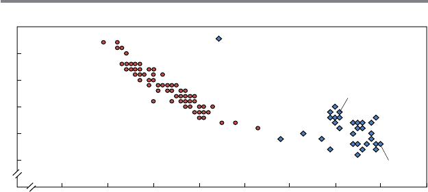
200 Brookings Papers on Economic Activity, Fall 2011

curve counterclockwise during a recession, and so the rise in structural

unemployment suggested by the current Beveridge curve is perhaps on the

order of 1 percentage point.

Of course, this discussion of the Beveridge curve raises precisely the

problem faced by Rothstein and others who have examined the relation-

ship between UI beneﬁts and unemployment. Because Congress extends

UI beneﬁts at times when aggregate demand is weak, it is difﬁcult to dis-

tinguish the rise in the unemployment rate induced by the extension from

the rise due to the lack of demand for labor.

How does Rothstein attack the problem? His basic approach is to care-

fully model the institutional details of the UI program and to adopt a vari-

ety of identiﬁcation strategies to estimate its effects, which allows him to

test the robustness of the results. He also decomposes the total impact of

extended UI beneﬁts on unemployment into a part due to the impact on

labor force participation and a part due to the impact on employment. This

decomposition is helpful because it gets at the question of whether eco-

nomic activity is being hampered by the program. It is also worth noting

one thing that Rothstein does not do, which is to use information from past

episodes in which beneﬁts were extended. This is important because, rela-

tive to previous episodes, the contraction that precipitated the recent exten-

sion was unusually prolonged and the recovery has been relatively anemic.

This suggests that the behavioral response could be different than in the

past. In addition, the 1994 redesign of the Current Population Survey (see

my note 1) may limit the usefulness of previous episodes.

Figure 3. Beveridge Curve, December 2000–October 2011

Unemployment rate

1.5

2.0

2.5

3.0

3.5

3.0 5.04.0 7.06.0 8.0 10.09.0

Sources: Job Openings and Labor Turnover Survey and Current Population Survey.

Job vacancy rate

Jan. 2009

2009-11 monthly observations

Oct. 2009

Jun. 2011

Of the four identiﬁcation strategies Rothstein uses, I will focus on

three. The ﬁrst uses variation in the availability of UI beneﬁts due to stops

and starts in program implementation, controlling for labor demand. The

expansion of the UI program responded not only to economic conditions,

but also to the exigencies of the political process. Congress regularly let

the program expire, and renewals were always uncertain. Finally, states

could choose whether to participate in the extended beneﬁts (EB) por-

tion of the program. These idiosyncrasies in implementation break the

link between economic conditions and the duration of available beneﬁts.

Although Rothstein models all these institutional details carefully, his use

of state unemployment rates to control for economic conditions raises a

problem: even with these controls (and controls for state ﬁxed effects),

there could be an omitted variable relating to the political economy of a

state—for example, the availability of other beneﬁts—that both contrib-

utes to the availability of EB and affects the probability that people remain

unemployed.

What Rothstein denotes as his third identiﬁcation strategy is very similar

to the one just described but adds controls for the estimated duration of the

federal component of the UI expansion, called emergency unemployment

compensation (EUC). He also adds control functions that model the indi-

vidual state EB triggers. This leaves variation in the state adoption of EB

as the only source of identiﬁcation. It is worth noting that this speciﬁcation

does increase the estimated impact of the UI extensions on labor force deci-

sions. In particular, the impact on the average exit hazard in 2010Q4 rises

from about 2 percentage points in the various speciﬁcations that follow the

ﬁrst identiﬁcation strategy to about 3 percentage points in this one.

A third identiﬁcation strategy (the second in the order in which the

paper presents them) is to use voluntary job leavers as a control group.

The problem here is that people who leave their job but remain in the

labor force must have information that the researcher does not about

their job opportunities or their willingness to drop out of the labor force;

these individuals likely have better opportunities or are more willing to

exit the labor force than a similarly situated person who has been laid

off. Rothstein is well aware of the problems with this approach and takes a

number of steps to control for the differences between the two groups that

one can observe: his regressions include as controls an estimated duration

of UI beneﬁts for the job leavers and a variety of individual covariates.

In addition, the inclusion of job leavers allows Rothstein to include state-

month ﬁxed effects. This actually enables him to control for the omit-

ted variable that, as I proposed above, could be correlated with both an

COMMENTS and DISCUSSION 201

202 Brookings Papers on Economic Activity, Fall 2011

individual’s decision to receive UI and the state’s decision to offer EB.

Interestingly, the estimated effect of the UI extensions is smaller in the

speciﬁcations identiﬁed using this third strategy (the average reduction in

the 2010Q4 exit hazard falls to about 1 percentage point), although, per-

haps unsurprisingly given the amount of variation soaked up by the state-

month ﬁxed effects, the coefﬁcients are less precisely estimated than in

other speciﬁcations. Despite Rothstein’s considerable work on this speci-

ﬁcation, I have mixed feelings about it. On the one hand, it seems that

despite the individual controls, there must still be unobserved differences

between job losers and job leavers that affect the probability of exit from

unemployment. On the other hand, the inclusion of the state-month ﬁxed

effects seems desirable, even if their usefulness is limited somewhat by

the reduction in power.

Having identiﬁed the impact of UI extensions on unemployment exit

hazards, Rothstein turns to decomposing this effect into changes due to

reemployment probabilities and changes due to labor force exit. For this

he uses multinomial logits. However, as he himself notes, the IIA (inde-

pendence of irrelevant alternatives) assumption implicit in a multinomial

logit is likely to be violated. The problem is that the choice between being

unemployed and exiting the labor force is not completely clear for the

marginal displaced worker—it is likely to be a matter of search effort.

But UI extensions probably have a particularly large impact on people who

would otherwise have exited because their reemployment probabilities

are low. As a result, the extensions could appear to depress reemployment

probabilities simply by increasing the share of the unemployment pool

that is less employable. Rothstein attempts to ameliorate this problem by

including a standard set of controls for personal characteristics. Although

these may help, the differences in search effort are likely driven by unob-

served heterogeneity. For this reason an alternative (albeit computationally

more costly) estimation strategy is probably worth pursuing. In particular,

Rothstein could have used multinomial probits, which do not require the

IIA assumption, or multinomial logits with random effects, which would

absorb some of the unobserved heterogeneity. In the absence of results

from one of these alternative techniques, I hesitate to put too much weight

on these results (or the analogous results dividing the unemployment rate

effect of UI extensions into parts due to reemployment and labor force

exit), although I ﬁnd them suggestive.

The penultimate section of the paper maps the estimated effect of UI

extensions on exit hazards onto effects on the stocks of the unemployed.

To accomplish this, Rothstein statistically forces the survival rates derived

COMMENTS and DISCUSSION 203

from the transitions observed in the matched monthly CPS to equal the

survival rates reported by respondents. This raises the question of whether

one should trust the reported durations more than the transition-derived

durations.

There are a number of obvious problems with the reported durations. First,

they are subject to substantial recall bias. Rothstein provides evidence from

the matched CPS data that people who report new spells of unemploy-

ment often report durations longer than is consistent with their observed

history. Moreover, a quick look at ﬁgure 7 of Rothstein’s paper shows

substantial heaping of responses at certain durations, which suggests that

recall bias is important. In addition, there is the problem of dependent cod-

ing of the monthly CPS: if a person who is unemployed in one month is

determined to be unemployed in the next, that person’s duration is automati-

cally increased by 4 weeks, regardless of whether he or she was unemployed

the whole time.

In contrast, some of the criticisms leveled against the transition-based

survival hazards are not particularly relevant. For instance, with regard to

the dependent coding, it has been argued that even if individuals actually

experience a short spell of employment or nonparticipation between sur-

veys, this is not a meaningful exit from unemployment, and therefore it is

not a problem for them to have been counted as unemployed for the entire

period. However, even if a person is actually out of work for the reported

duration, he or she might not have been unemployed by the CPS deﬁni-

tion, which is what one is trying to match. Rothstein also presents evidence

from validation studies done in the 1980s showing signiﬁcant numbers of

spurious transitions. However, one goal of the 1994 CPS redesign was to

improve the identiﬁcation of labor market status, and there is evidence in

papers by Bureau of Labor Statistics (BLS) staff at the time that it did

improve their ability to consistently identify unemployment. Therefore,

validation studies from the 1980s criticizing the transitions are not so rel-

evant. Here I should point out that Rothstein did talk to staff at the BLS to

obtain updated information on the validity of the transitions reported in the

monthly CPS, but the BLS would not release the data. Finally, it should

be noted that even the monthly ﬂows understate transitions. Christopher

Nekarda (2009), using weekly data from the Survey of Income and Pro-

gram Participation, ﬁnds that gross ﬂows are understated by 15 to 24 per-

cent in monthly data. This does not suggest that one’s prior should be that

U-N-U and U-E-U transitions are spurious.

Unfortunately, Rothstein does not test the robustness of his results to

forcing the survival curve from the ﬂow data to look like that from the

204 Brookings Papers on Economic Activity, Fall 2011

reported durations, although he does present two different methods of

reconciling the curves. From private correspondence, I think he believes

he would ﬁnd even smaller results using the transition-based dura-

tions. Nonetheless, I would have liked to see a robustness check of this

assumption.

All that said, I found the results that UI extensions have had a small

impact on the unemployment rate in the recent recession and recovery

compelling. Rothstein uses a variety of identiﬁcation strategies to estimate

his results and subjects them to numerous speciﬁcation tests. Moreover, the

simple fact that Rothstein estimates, rather than extrapolates, the results,

and the care with which he performs the analysis, make this an important

contribution to the literature. Although his results are on the low side of

other estimates, they are not orders of magnitude different from those of

other carefully performed analyses, even those that do extrapolate. Whether

the UI program has raised the unemployment rate by 0.2 percentage point

or 1 percentage point (or somewhere in between, as I suspect), the fact is

that extended UI beneﬁts can explain only a small portion of the rise in the

unemployment rate since the recession.

By itself the paper cannot answer the question I raised at the outset:

whether the current increase in the unemployment rate is due to a shortfall

in aggregate demand or to a rise in structural factors. However, the ﬁnd-

ing does eliminate one potential cause of higher structural unemployment.

Moreover, the fact that the impact of the UI extensions program is small

argues in favor of extending UI beneﬁts as part of a ﬁscal stimulus package,

since it helps families in need and has a high multiplier, with only a small

downside.

REFERENCES FOR THE AARONSON COMMENT

Barnichon, Regis, and Andrew Figura. 2010. “What Drives Movements in the

Unemployment Rate? A Decomposition of the Beveridge Curve.” Finance and

Economics Discussion Series no. 2010-48. Washington: Board of Governors of

the Federal Reserve System.

Nekarda, Christopher J. 2009. “Understanding Unemployment Dynamics: The

Role of Time Aggregation.” Washington: Board of Governors of the Federal

Reserve System (June).

3. Rothstein does test whether the decision to exclude individuals with U-E-U and

U-N-U transitions biases the results of his hazard rate models. The estimated effects of UI on

the hazard rates are a bit larger, but of the same order of magnitude.

Polivka, Anne E., and Stephen M. Miller. 1998. “The CPS after the Redesign:

Refocusing the Economic Lens.” In Labor Statistics Measurement Issues,

edited by John Haltiwanger and others. University of Chicago Press.

COMMENT BY

LISA B. KAHN In this paper Jesse Rothstein asks whether the recent

extensions to unemployment insurance (UI) beneﬁts have led to an increase

in the unemployment rate. Basic agency theory suggests that subsidizing

unemployment creates a disincentive for workers to search for jobs. How-

ever, it is unclear whether, in a period of severely depressed labor demand,

this moral hazard imposes so large a cost as to outweigh the many beneﬁts

associated with UI extensions. Rothstein ﬁnds that the recent incarnations

of the Emergency Unemployment Compensation (EUC) and Extended

Beneﬁts (EB) programs have had only small impacts on the overall unem-

ployment rate, raising it by 0.1 to 0.5 percentage point. He shows that the

bulk of the effect is in dissuading unemployed workers from exiting the

labor force, with a smaller share being driven by reduced reemployment

rates. His ﬁndings are remarkably robust to four different identiﬁcation

strategies.

The impact of UI on a worker’s labor supply is one of the most important

questions facing policymakers today. The EUC and EB programs, which

currently extend UI coverage from 26 weeks to potentially 99 weeks, are

frequently up for renewal and thus continuously in need of justiﬁcation.

However, previous research serves as only a rough guide to the cost-beneﬁt

analysis of these programs.

An older literature on the impacts of UI on job search produced a wide

range of estimates that are quite out of date. The gold standard approaches

were those of Lawrence Katz and Bruce Meyer (1990) and Robert Mofﬁtt

(1985), who exploited the observation of a large spike in the probabil-

ity of exiting unemployment in the last week of coverage, and the natu-

ral experiment approach of David Card and Philip Levine (2000). Katz

(2010) himself points out that labor market institutions such as temporary

layoffs and recalls have changed substantially since the period most of

these papers study. Further, the methodology exploited in most of the pre-

vious literature did not allow for separate estimates of the impacts of UI

on reemployment and labor force exit. Especially for policy, the distinc-

tion is important.

In response to renewed policy interest in this question, a new itera-

tion of papers has emerged. One strand extrapolates from the previous

COMMENTS and DISCUSSION 205

206 Brookings Papers on Economic Activity, Fall 2011

literature, and for the reasons stated above, its results can be quite mis-

leading. Meanwhile many of the regional Federal Reserve banks have

quickly ﬁlled policymakers’ need for up-to-date research with clever

back-of-the-envelope calculations. Their estimated impacts of UI exten-

sions on the unemployment rate range from about 0.4 to 2.0 percentage

points (Aaronson, Mazumder, and Schechter 2010, Fujita 2010, Valletta

and Kuang 2010). These papers helpfully provided reasonable, relatively

consistent estimates in a hurry.

However, the literature still cried out for systematic econometric studies

performed on data contemporaneous to the crisis. Rothstein provides this.

His approach is able to estimate the separate impacts of UI on reemploy-

ment and labor force exit—a distinction that matters for policymakers, and

one that many of the previous papers were not able to make. He makes

extremely careful use of longitudinally linked Current Population Survey

data. He very carefully considers sources of variation in UI beneﬁt dura-

tions, a point that I discuss in more detail below. Finally, his results pass

the smell test: he ﬁnds some evidence for moral hazard, which aligns with

economic theory, but he also ﬁnds that the distortions are small, as the cur-

rent distressed state of labor demand might suggest.

The difﬁculty in studying this problem is that beneﬁts are extended at

precisely the moment when job ﬁnding rates fall. Rothstein’s approach to

dealing with this problem is a veritable kitchen sink, exploiting four dif-

ferent sources of variation. He mainly exploits discrete changes in maxi-

mum beneﬁt length based on triggers that vary across states and over time,

allowing him to control for changes in local labor market conditions. The

downside is that no single approach is perfect; each requires somewhat

unpalatable assumptions. For example, in some speciﬁcations he must para-

metrically control for economic conditions, whereas in others he exploits

cross-sectional variation in UI eligibility and can control for state-month

ﬁxed effects. The latter strategy alleviates reliance on functional form but

requires the assumption that those ineligible for UI are a good control group

for the eligible. The assumptions thus differ across approaches, yet each

approach yields estimates that are remarkably consistent with the others.

This suggests that no one assumption can be driving the results, so that one

feels better about the overall package.

The regressions reported in the paper take the form of a job ﬁnding

hazard on the left-hand side and expected beneﬁt duration on the right,

1. So do Farber and Valletta (2011) in a contemporaneously written paper.

COMMENTS and DISCUSSION 207

along with several different controls for current labor market conditions.

The main difﬁculty, as I see it, is in measuring the length of time unem-

ployed workers expect to receive beneﬁts. Rothstein equates expectations

with current law, assuming that workers expect no further action by Con-

gress to extend beneﬁts. Henry Farber and Robert Valletta (2011) obtain

similar results with the opposite approach, one that assumes that current

law will be extended throughout the worker’s UI duration. Both assump-

tions are reasonable, but both will suffer from measurement error since it is

impossible to capture true expectations.

This means that the main coefﬁcient suffers from attenuation bias. More-

over, the problem is worse than that since, for a given worker, the accuracy

of this proxy for expectations will change over time. In particular, as unem-

ployment duration increases, current law probably becomes a more accurate

predictor of a worker’s expectations.

For example, consider a worker who became unemployed in January

2010 and lived in a state with 99 weeks of UI. At that point Rothstein’s mea-

sure of expected duration for that worker, D

its

, would have been 46 weeks

(26 weeks of regular UI coverage and 20 weeks of EB), since the EUC

program was scheduled to sunset later that winter.

By late July 2010, if the

worker were still unemployed, D

its

would have included one tier of EUC,

since the program was reauthorized through November 2010. In Decem-

ber, when all four EUC tiers were reauthorized until January 2012, D

its

for

this worker would have been the full 99 weeks. Ex post, we know that this

worker would be eligible for 99 weeks of UI, but Rothstein’s measure would

have only incorporated this about a year into the UI spell. It is unclear what

the worker’s expectations would have been throughout the spell. However,

both Rothstein’s measure and the worker’s expectations would have been

most accurate toward the end of the 99 weeks.

The attenuation bias generated by this measurement error is a bigger

problem for workers with low durations of unemployment than for those

with high durations. This could be why Rothstein ﬁnds effects that are

almost always larger in magnitude for those with more than 26 weeks of

unemployment. He addresses this problem as best he can, with some robust-

ness checks. But it is worth thinking about whether this measurement error

problem causes him to slightly understate the impact of UI extensions on

the unemployment rate.

2. In fact, the worker might have expected only 26 weeks, since many states also had

automatic triggers that would end their EB programs when 100 percent federal funding

expired along with the EUC program.

208 Brookings Papers on Economic Activity, Fall 2011

Despite the problem of measurement error, I believe this paper estab-

lishes quite well that in the current economy, UI extensions pose minimal

consequences to job search behavior. Given that conclusion, it is worth

thinking next about the beneﬁts that UI provides, and in particular the ben-

eﬁts of extending UI in an economic slump. Rothstein, rightly, does not

expound on these issues in his paper; he sets out a speciﬁc, important ques-

tion and answers it well. In the rest of this comment, I will touch on some

of the issues beyond the scope of his paper, including the value of the extra

search time that UI provides unemployed workers and the value of UI as

economic stimulus.

It has been commonly suggested that UI allows workers more time to

search for the right job, thus helping them ﬁnd better matches. Recent

evidence suggests that the stakes to ﬁnding the right job are particularly

high in recessions. In their paper in this volume, Steven Davis and Till von

Wachter summarize and provide new evidence on the long-term costs of

job displacement, ﬁnding that the effects are particularly large and damag-

ing when displacement comes in a recession. Further, a growing body of

work ﬁnds that workers who graduate from school in a downturn receive

on average, lower wages, which persist long into their careers, even though

they spend little time in unemployment (Kahn 2010, Oreopoulos, von

Wachter, and Heisz 2012, Oyer 2008).

These ﬁndings suggest that having to search for work during an eco-

nomic slump is particularly damaging. Indeed, job matches in recessions

are typically of lower quality and in worse ﬁrms (Bowlus 1995, Davis,

Haltiwanger, and Schuh 1996). Furthermore, in recent work (Kahn 2011)

I have shown that despite ending up in worse jobs, workers who take jobs

in a downturn actually stay in those jobs longer than do other workers at

the same ﬁrm. It is unclear what mechanism drives these results, but they

do suggest that job placement in a downturn is crucial to future success.

Extensions to UI allow workers some ﬂexibility toward putting themselves

in the best job possible.

A report by the Council of Economic Advisers (2010) estimates that as of

2010Q3, 40 million people had beneﬁted from EUC or EB either as recipi-

ents themselves or through receipt by household members. In 42 percent of

these families, UI was essentially the only source of income. In addition to

the private beneﬁts associated with UI, the extensions beneﬁt the economy

as a whole. EUC and EB are a particularly well-targeted form of economic

stimulus, since they go to people who are very likely to spend the money

(Elmendorf 2010). They may also help keep workers off of disability insur-

ance, a typically irreversible transition (Autor and Duggan 2006), and may

COMMENTS and DISCUSSION 209

help avoid mortgage foreclosures (Foote and others 2009). These beneﬁts

are important to keep in mind when weighing the costs and beneﬁts of

extending UI.

As of this writing (October 2011), labor demand is still severely

depressed. There are almost 14 million unemployed, including almost 6 mil-

lion long-term unemployed, in addition to the 1 million discouraged

workers who have exited the labor force but will, one hopes, reenter at

some point. Posted vacancy rates hover at low levels that imply more than

four job seekers per job opening. Unemployed workers thus need more

time to ﬁnd jobs than they would during normal times; indeed, job ﬁnding

rates are about half what they were in good times and have not recovered

any ground. UI gives these workers much-needed support. Rothstein’s

paper contributes to a growing body of evidence that distortions to job

search behavior caused by UI are much lower in recessions (see also Kroft

and Notowidigdo 2011 and Schmieder, von Wachter, and Bender forthcom-

ing). This evidence should weigh heavily in the policy debate on whether

the UI extensions should be renewed in the course of 2012 and beyond.

REFERENCES FOR THE KAHN COMMENT

Aaronson, Daniel, Bhashkar Mazumder, and Shani Schechter. 2010. “What Is

behind the Rise in Long-Term Unemployment?” Federal Reserve Bank of Chi-

cago Economic Perspectives 34, no. 2: 28–51.

Autor, David H., and Mark G. Duggan. 2000. “The Growth in the Social Security

Disability Rolls: A Fiscal Crisis Unfolding.” Journal of Economic Perspectives

14, no. 3: 37–56.

Bowlus, Audra J. 1995. “Matching Workers and Jobs: Cyclical Fluctuations in

Match Quality.” Journal of Labor Economics 13, no. 2: 335–50.

Card, David, and Philip B. Levine. 2007. “Extended Beneﬁts and the Duration of

UI Spells: Evidence from the New Jersey Extended Beneﬁt Program.” Journal

of Public Economics 78, nos. 1-2: 107–38.

Council of Economic Advisers. 2010. “The Economic Impact of Recent Temporary

Unemployment Insurance Extensions.” Washington (December).

Davis, Steven, John Haltiwanger, and Scott Schuh. 1996. Job Creation and Destruc-

tion. MIT Press.

Elmendorf, Douglas. 2010. “Policies for Increasing Economic Growth and Employ-

ment in the Short Term.” Testimony prepared for the Joint Economic Committee

of the United States Congress, February 23. Washington: Congressional Budget

Ofﬁce.

Farber, Henry S., and Robert Valletta. 2011. “Extended Unemployment Insurance

and Unemployment Durations in the Great Recession: The U.S. Experience.”

Princeton University and Federal Reserve Bank of San Francisco (June 24).

210 Brookings Papers on Economic Activity, Fall 2011

Foote, Christopher L., Kristopher S. Gerardi, Lorenz Goette, and Paul S. Willen.

2009. “Reducing Foreclosures: No Easy Answers.” NBER Macroeconomics

Annual 24: 89–138.

Fujita, Shigeru. 2010. “Economic Effects of the Unemployment Insurance Ben-

eﬁt.” 2010. Federal Reserve Bank of Philadelphia Business Review (Fourth

Quarter) 20–27.

Kahn, Lisa B. 2010. “The Long-Term Labor Market Consequences of Graduating

from College in a Bad Economy.” Labour Economics 17, no. 2: 303–16.

_________. 2011. “Job Durations, Match Quality and the Business Cycle: What

We Can Learn from Firm Fixed Effects.” Yale University.

Katz, Lawrence F. 2010. “Long-Term Unemployment in the Great Recession.”

Testimony prepared for the Joint Economic Committee. Harvard University

(April 28).

Katz, Lawrence F., and Bruce D. Meyer. 1990. “Unemployment Insurance, Recall

Expectations, and Unemployment Outcomes.” Quarterly Journal of Economics

105, no. 4: 973–1002.

Kroft, Kory, and Matthew J. Notowidigdo. 2011. “Should Unemployment Insur-

ance Vary with the Unemployment Rate? Theory and Evidence.” Working Paper

no. 17173. Cambridge, Mass.: National Bureau of Economic Research (June).

Mofﬁtt, Robert A. 1985. “Unemployment Insurance and the Distribution of Unem-

ployment Spells.” Journal of Econometrics 28: 85–101.

Oreopoulos, Phil, Till von Wachter, and Andrew Heisz. 2012. “The Short- and

Long-Term Career Effects of Graduating in a Recession: Hysteresis and Het-

erogeneity in the Market for College Graduates.” American Economic Journal:

Applied Economics 4: 1–29.

Oyer, Paul. 2008. “The Making of an Investment Banker: Macroeconomic Shocks,

Career Choice, and Lifetime Income.” Journal of Finance 63: 2601–28.

Schmieder, Johannes F., Till von Wachter, and Stefan Bender. Forthcoming. “The

Effects of Extended Unemployment Insurance over the Business Cycle: Evi-

dence from Regression Discontinuity Estimates over Twenty Years.” Quarterly

Journal of Economics.

Valletta, Rob, and Katherine Kuang. 2010. “Extended Unemployment and UI Ben-

eﬁts.” FRBSF Economic Letter No. 2010(12) (April). Federal Reserve Bank of

San Francisco.

GENERAL DISCUSSION Jeffrey Kling recalled that previous work

by Daron Acemoglu and Robert Shimer had suggested that unemploy-

ment insurance can facilitate mobility to new occupations by providing a

safety net if job transitions do not work out—which may also lead to better

matches between workers and jobs. He also reiterated Lisa Kahn’s concern

about worker mobility as a potential source of error in the analysis, since

the CPS tracks households and not individuals, who may move between

households. Jesse Rothstein replied that he had not examined data on

COMMENTS and DISCUSSION 211

wages upon reemployment that would provide evidence about the quality of

matches; he was fairly conﬁdent that the mobility issue was not corrupting

his results but acknowledged he needed to add more statistics to support that.

Robert Hall questioned Rothstein’s use of reemployment hazard rates

in his econometric framework, given the structure of errors in employment

data in the CPS. Errors arise when respondents do not classify themselves

in accordance with the technical deﬁnitions of “employed,” “unemployed,”

and “not in the labor force.” He noted a feature of the CPS that may exac-

erbate reporting error: not every person in the CPS is interviewed directly;

rather, a single respondent is designated to respond for all members of the

household. Hall suggested that instead of calculating hazard rates, which

amounts to taking ﬁrst differences of the data, Rothstein come up with an

indirect inference approach more clearly based on the theoretical model of

unemployment he presented in the paper, even though such an approach

would represent a signiﬁcant departure from previous literature.

Hall pointed out further that a large recent drop in job matching efﬁ-

ciency remained unexplained. He saw Rothstein’s results as compelling

evidence that unemployment insurance does not explain this drop, which

leaves open the question of what does. Hall also asked whether Steven

Davis could comment on the possible sources of recent deviations from

the historical Beveridge curve, which is meant to measure changes in labor

market efﬁciency.

Responding to Hall, Steven Davis cited two pieces of evidence about

the sources of recent deviations from the historical Beveridge curve and

the recent breakdown in the empirical relationships implied by a standard

matching function. First, in work with John Haltiwanger and Jason Faber-

man, Davis found that the intensity of recruitment to ﬁll vacant positions

had declined sharply during the recent recession and remains low. Second,

a recent Brookings Paper by Alan Krueger and Andreas Mueller found that

job search intensity declines with the duration of an unemployment spell.

In his comment on that paper, Davis showed that their evidence, combined

with the recent increase in average spell durations at the aggregate level,

implies a sizable drop in search intensity per unemployed person.

Rothstein suggested that the decline in matching efﬁciency was driven

by the very low level of job openings. Matching theory posits a frictional

rate of job vacancies, and Rothstein thought that for a period during the

recession, the vacancy rate had fallen below the frictional level. For a

while, therefore, the matching rate might have fallen even though people

were searching harder for jobs, because there were so few job openings.

This interpretation led Rothstein to doubt the need for new models to

212 Brookings Papers on Economic Activity, Fall 2011

describe a breakdown in the job matching process. Such an exercise, he

thought, would require too much extrapolation from previous circumstances

to provide new insights.

Davis also hoped that someone would apply Rothstein’s methodology

to previous extensions of UI, to see whether UI had different effects in

different macroeconomic environments. He thought that both the policy

debate and academic research dwelled too much on the question of whether

UI extensions are good or bad; lawmakers and researchers should instead

spend more time evaluating the beneﬁts and costs of UI extensions against

alternative policy options, especially since UI extensions are expensive.

Davis expressed disappointment at the federal government’s willingness to

legislate additional expenditure on UI without encouraging states to con-

duct randomized controlled experiments on alternative ways to help the

unemployed, especially the long-term unemployed, get back to work. In his

view, setting aside the macroeconomic effects, the main welfare beneﬁt of

UI comes from its income and consumption smoothing effects. Two alter-

native policies might achieve the same effects at lower cost: workers could

make some type of prepayment, building up funds to be drawn on during

spells of unemployment, or the government could offer low-cost loans to

unemployed workers, to be repaid when they are once again employed.

Rothstein disagreed, on the grounds that a prepayment or loan plan would

be no less expensive than UI but would simply be accounted for differently. He

argued that, aside from whatever moral hazard they create, both UI and these

alternative policies amount to transfer programs. People can differ on the mer-

its of the transfer, but economic analysis can only lend insight into the costs of

moral hazard and any other incentive distortions created by the policies.

George Akerlof seconded a point that Kahn had made about interpreting

the welfare impact of UI. If one considers the labor market to be a rationed

market, then a subsidy in the market has a positive impact on welfare. By

enabling unemployed workers to search longer rather than take the ﬁrst job

offered, UI enables them to ﬁnd a better match. He reminded the Panel that

another beneﬁt of UI in recessions is that it provides economic stimulus by

putting money in the hands of people who will spend it. Rothstein replied

that he had not spent much time investigating the impact of UI extensions

on job match quality because earlier research had not found a relationship

between the two.

Till von Wachter suggested that past empirical research on UI extensions

had been unclear about whether it was measuring pure partial equilibrium

effects or general equilibrium effects. Like these earlier papers, Rothstein’s

estimates actually represented a hybrid of partial and general equilibrium

COMMENTS and DISCUSSION 213

effects, because they exploited both state variation and time variation in

UI availability over a period during which economic conditions were also

changing. Von Wachter also revisited Rothstein’s point that back-of-the-

envelope extrapolations from prerecession estimates far overestimated the

impact of UI extensions on unemployment. He noted that straightforward

adjustments to these extrapolations, such as allowing for congestion in the

labor market, imperfect take-up of UI beneﬁts, or low job arrival rates,

could produce estimates much closer to Rothstein’s results.

Finally, von Wachter sought to clarify a point on the implications of a

paper he had written with Johannes Schmieder and Stefan Bender on the

varying effects of extended UI over the business cycle. Using 25 years of

unemployment data from Germany and a clean identiﬁcation strategy, they

had found that rates of exhaustion of UI rose sharply during recessions,

but that the effect of UI on the probability of regaining employment stayed

constant over the business cycle. The upshot of these two facts, he argued,

is that the moral hazard effect of UI falls during recessions, providing a

clear rationale for extending UI during economic slumps.

Ricardo Reis pointed out what seemed to him a contradiction between

Rothstein’s results and previous research. An extensive literature from the

1990s had shown, using cross-country comparisons, that high levels and

durations of UI beneﬁts helped explain the high levels of unemployment

in some European countries. Reis argued that, in theory, a rule promising

extended UI beneﬁts during a recession should have the same effect on

unemployment as a higher level of UI beneﬁts throughout the business

cycle, but Rothstein’s results suggested this was not the case.

John Quiggin thought it bizarre that the political debate focused so much

on the moral hazard effects of UI beneﬁt extensions. He saw the potential

for much costlier moral hazard among people who had exhausted their

UI beneﬁts and sought disability insurance, since those who successfully

apply for DI seldom return to the labor force and instead receive beneﬁts

for the rest of their lives. Rothstein said he planned to look more into the

relationship between UI and DI using data on DI income from the CPS.

Betsey Stevenson noted that President Obama’s proposed American Jobs

Act called for spending $5 billion on experiments aimed at getting long-

term unemployed workers back to work. She also reminded the Panel of

how few people are actually eligible for UI: currently about a quarter of

the unemployed received state-based UI, and another quarter received UI

through the federal extensions, leaving half of the unemployed without ben-

eﬁts at all. She inferred that if UI reduces job search intensity among recipi-

ents, it should skew job-ﬁnding rates in favor of those who are ineligible.