What Effects Did United Airlines' De-Hubbing of Cleveland Hopkins International Airport Have on Cleveland Passengers?

Colby College Colby College

Digital Commons @ Colby Digital Commons @ Colby

Honors Theses Student Research

2018

What Effects Did United Airlines' De-Hubbing of Cleveland What Effects Did United Airlines' De-Hubbing of Cleveland

Hopkins International Airport Have on Cleveland Passengers? Hopkins International Airport Have on Cleveland Passengers?

Joshua A. Young

Colby College

Follow this and additional works at: https://digitalcommons.colby.edu/honorstheses

Part of the Economics Commons

Colby College theses are protected by copyright. They may be viewed or downloaded from this

site for the purposes of research and scholarship. Reproduction or distribution for commercial

purposes is prohibited without written permission of the author.

Recommended Citation Recommended Citation

Young, Joshua A., "What Effects Did United Airlines' De-Hubbing of Cleveland Hopkins

International Airport Have on Cleveland Passengers?" (2018).

Honors Theses.

Paper 901.

https://digitalcommons.colby.edu/honorstheses/901

This Honors Thesis (Open Access) is brought to you for free and open access by the Student Research at Digital

Commons @ Colby. It has been accepted for inclusion in Honors Theses by an authorized administrator of Digital

Commons @ Colby.

What Effects Did United Airlines' De-Hubbing

of Cleveland Hopkins International Airport

Have on Cleveland Passengers?

Joshua A. Young

Honors Thesis

Department of Economics

Colby College

April 26, 2018

Advisor: Professor Timothy P. Hubbard

Reader: Professor Samara R. Gunter

Abstract

This paper uncovers the effects on passengers from United Airlines’ 2014 de-hubbing of

Cleveland Hopkins International Airport (CLE). Airline networks are often reorganized for

efficiency; during the process, an airport may gain or lose hub operations, affecting passengers in

different ways depending on the market environment. I take an empirical approach using

difference-in-differences models to analyze 28 quarters of Bureau of Transportation Statistics

data. I find that de-hubbing contributed to significant reductions in airfare per mile out of CLE.

This is consistent with past cases of de-hubbing where low-cost carriers were present. However,

quality measures, including the number of nonstop destinations served and on-time performance,

were harmed.

I. Introduction

The hub-and-spoke network is commonplace in post-deregulation airline networks, and

travelers frequently stop at a hub to change planes and catch a connecting flight to reach their

final destinations. Legacy carriers favor a hub-and-spoke network where each airline has

multiple hub airports located around the country. An airport has hub status when it hosts a

dominant airline that concentrates traffic there, routing demand from multiple “spoke” airports

through the hub airport to maximize efficiency. Following a significant change such as a merger,

a hub airline may make the strategic decision to reorganize its network and de-hub an airport by

significantly reducing capacity and the number of spoke routes serviced. There have been

multiple recent cases of de-hubbing. American de-hubbed operations at Lambert-St. Louis

International Airport in 2004. Delta ceased hub operations at Dallas/Fort Worth International

Airport in 2005 and a year later de-hubbed Cincinnati/Northern Kentucky International Airport

(Tan & Samuel, 2016). In 2013, Delta scaled down departures at Memphis International Airport

to just below hub levels (Mutzabaugh, 2013).

Observational evidence suggests that the effects of de-hubbing on price and quality are

unclear and move in different directions depending on airport characteristics and network

environment. Understanding the impacts of de-hubbing is, therefore, an empirical question to be

explored with real-world data. United Airlines de-hubbed Cleveland Hopkins International

Airport (CLE) in 2014 and committed to 60% fewer departures after acquiring the hub in a 2010

merger with Continental Airlines. We consider the case of de-hubbing Cleveland because it is

the most recent example of an airport to lose its hub status. Hubs are essential parts of a local

economy, generating hundreds of jobs and revenue for a city. When United left, people lost jobs

in Cleveland. Are all consequences of de-hubbing negative, or did passengers benefit in any

way? CLE should have an informative story to tell and provide a means to contribute to our

understanding of the effects caused by de-hubbing on a range of passenger-specific and market

factors including airfare per mile, quality measured by flight frequency and the number of

destinations offered, market concentration, on-time performance, and rival response.

While existing empirical studies on de-hubbing have considered airport-wide effects and

multiple de-hubbed airports in their analyses, I instead take a narrower but more comprehensive

approach with the case of CLE, exploring both immediate and subsequent effects of de-hubbing

at the biannual and quarterly levels using a difference-in-differences approach. Because United’s

de-hubbing of CLE is recent, analysis of CLE is uncommon in the literature. I use

comprehensive data from the Bureau of Transportation Statistics which allows for in-depth

analyses and exploration of recovery patterns.

I find that United’s de-hubbing of CLE contributed to reduced prices for nonstop CLE

passengers. The largest magnitude reduction took place one year after de-hubbing finished where

there was a statistically significant 12.2% decrease in average airfare per mile for flights

departing CLE in the second half of 2015 relative to the second half of 2013. Empirical evidence

shows that low-cost carriers, Frontier and Spirit, expanded their operations at CLE following de-

hubbing. Low-cost carriers offer reduced quality but also lower fares than legacy carriers, such

as United, therefore putting downward pressure on prices in 2015. Subsequently, as the amount

of seat capacity departing CLE recovered, airfare per mile returned to pre-de-hubbing levels.

Further results show that nonstop passengers from CLE experienced reduced quality with a 53%

reduction in the number of destinations offered immediately following de-hubbing compared

with what United offered before. The frequency of flights was also reduced and did not

completely recover. My analyses provide no clear conclusion for changes in on-time

performance; I do not find the fewer delays expected from alleviated congestion. As expected in

any de-hubbing scenario, United’s market power decreased, and market concentration at CLE

fell dramatically following de-hubbing. My results may be generalizable to other cases of de-

hubbing where the airport looks similar to CLE. My findings could also be relevant to antitrust

policy considering the impacts of consolidation in the airline industry – the de-hubbing of CLE

followed a merger but was characterized by a reduction in prices and market power, albeit with

adverse effects on nonstop travel quality.

II. United’s De-hubbing of CLE

United Airlines announced on May 3, 2010, that it would merge with Continental

Airlines in a $3.17 billion deal. Combined, the airlines would have 21% of domestic seat mile

capacity (Mouawad & Merced, 2010). Employee unions did not oppose the deal, and the merger

was approved by the U.S. Department of Justice on August 27, 2010, following the completion

of their antitrust review (United, 2010). On October 1, 2010, United and Continental announced

the successful completion of their merger (SEC, 2010), and one year later, after combining

operations, United received approval for a single operating certificate from the Federal Aviation

Administration on November 30, 2011. Passenger services were fully integrated by the first

quarter of 2012 (Peterson, 2011). During a press conference on the day of the announcement,

Jeff Smisek, chief executive of Continental at the time, said that the merger would allow the two

airlines to be successful in the dynamic and competitive airline industry. He suggested that the

two carriers would complement each other across markets and obtain synergies where one airline

was strong, and the other was weak (Smith, 2010).

During the merger, United adopted the small Cleveland Hopkins International Airport

(CLE) hub from Continental. However, as part of the network operations reorganization that

comes with a merger, CLE lost its hub status. Loss of hub designation is detrimental to many

different stakeholders including those in Cleveland. Jobs in the community suffer when traffic is

lower at airport facilities, and revenues fall. De-hubbing changes may affect consumer welfare.

Frequent flyers from Cleveland have fewer choices than before, and local businesses may be

harmed by the increased difficulty for travelers to reach them (Luo, 2014). United CEO Jeff

Smisek sent a letter to employees on February 1, 2014, obtained by local news outlet WKYC,

notifying them of the strategic decision to “substantially reduce [United’s] flying from

Cleveland.” Smisek cited the fact that United’s Cleveland hub “[had not] been profitable for over

a decade, and [had] generated tens of millions of dollars in annual losses in recent years.” He

wrote that there was insufficient demand for connecting flights through the hub, and United was

simply reacting to the nature of the market. Furthermore, new federal regulations at the time

adversely affected regional partner flying. According to the letter, the reduction in flights from

the de-hubbing process would occur beginning in April 2014 in one-third increments until

proposed reductions were fully realized in June of the same year. Smisek announced average

daily departures would be reduced by 60% – a more than 70% reduction in regional departures

(where United partners operate the regional flights under the United Express brand) with a

smaller reduction in mainline flights (where United is the operating carrier) – corresponding to a

reduction in available seat miles of 36%. Most departures out of CLE were United Express

flights before de-hubbing (Cho, 2014). A timeline of events is given below in Figure 1. Smisek

claimed it was a painful business decision given the impact on employees and loss of jobs

(WKYC, 2014). In the immediate aftermath, 470 workers directly involved in United’s

operations lost their jobs (Perkins, 2014). It is possible that other airlines have hired while

expanding their operation at CLE since then.

In a January 2015 article, less than one year after de-hubbing, Cleveland.com suggested

that passengers had been adversely affected by needing to travel longer routes and use more

connecting flights, even with the expanded presence of low-cost carriers. Local businesses, many

of which had relied on United, were also harmed due to lost employee productivity from

increased flying inconvenience. However, some businesses surveyed said that airfares had fallen

with increased low-cost options, something that likely would not have occurred while United

dominated CLE (Funk, 2015). A local WKSU article published in May 2016, reflected that the

predictions of a “devastating blow to the region” following the de-hubbing had not come to

fruition. Many of the major and popular vacation destination routes are still offered nonstop

because there is sufficient demand. Joe Roman of the Greater Cleveland partnership said that

having CLE as a hub would be preferable, but the available number of seats has risen almost

back to pre-de-hubbing levels since larger aircraft are being flown and other airlines have

expanded offerings at lower prices. However, travelers have significantly fewer options for direct

flights, so impacts on frequent flyers are disproportionately large from the increased travel time

Figure 1. Timeline of United’s merger with Continental and United’s de-hubbing of Cleveland airport.

and inconvenience (Niedermier, 2016). An additional WKSU report points to United’s de-

hubbing as still harming northeast Ohio’s largest firms. Diebold Corporation acknowledged that

business partners were not pleased with travel to CLE (Rudell, 2016). This anecdotal evidence is

supported by findings in Brueckner (2003) which links airline traffic to employment in U.S.

metropolitan areas. When an airport hosts frequent flights to and from a range of locations, local

businesses benefit, especially ones that require face-to-face meetings. Brueckner estimated that a

city could generate a 1% increase in service industry jobs with a 10% increase in enplanements.

Overall, whether or not an airport is a hub affects passengers, and also has implications for the

host city, its people, and the local economy.

III. Background on Deregulation, Hub Characteristics, Mergers, and De-Hubbing

Before considering the consequences of United’s de-hubbing of CLE, I provide

background on the history of deregulation that allowed CLE to be hubbed in the first place,

summarize airline pricing and costs, and review the characteristics of a hub-and-spoke network. I

also present an overview, supported by the literature, of airfare and quality at hub airports,

mergers, network organization, and de-hubbing.

Deregulation

In 1976 the Civil Aeronautics Board (CAB) began the process of deregulating the airline

industry following years of government intervention. Two years later, Congress passed the

Airline Deregulation Act, lifting a previous mandate which disallowed market competition in the

airline industry. Entry and price regulation were considerably relaxed, and market forces led to

new entrants, reducing prices. Hub-and-spoke network operations also grew in popularity.

Following deregulation, it did not take long for airlines to introduce frequent flyer and customer

loyalty programs, and the far reach of hub-and-spoke networks complemented those efforts

(Borenstein, 1992). According to Borenstein (1992), the biggest surprise two decades ago was

how fundamentally hub-and-spoke operations improved industry efficiency and changed the way

competition worked. We are still seeing the continuing effects of deregulation now – the initial

hubbing of CLE, the merger between United and Continental, and the de-hubbing of CLE are all

consequences of an airline industry with less regulation.

Carrier pricing and costs

With CAB no longer promoting simple fare structures, variation in prices across routes,

and even among what is paid by passengers on the same route, was expected. Travelers have

become familiar with how ticket prices change over time for a flight as the departure date nears,

and with demand during certain days or periods over the year. Fare dispersion has traditionally

been high, especially for legacy carriers with complex fare structures. However, now consumers

can see prices easily across carriers on the internet, and this may in part explain the dramatic fall

in intercarrier price dispersion (Borenstein & Rose, 2014). Given the relative importance of

competing on base fare, this could also explain the myriad of fees that passengers face, like

checked baggage fees. Loyalty programs help diminish price competition among carriers by

offering incentives to fly with one airline and impose switching costs to fly with another. Beyond

airfares, airlines face demand volatility, both predicted and stochastic, which leads to large

earnings volatility. High fixed costs accentuate the effects of variable demand. Airline labor

costs, including wages and benefits, are a significant cost factor averaging 35% of operating

costs between 1990 and 2007 (Borenstein & Rose, 2014). Airlines are not able to quickly reduce

or increase production capacity and change flight schedules. Accounting for variations in fuel

costs is also challenging. However, marginal costs are minimal for each additional passenger;

therefore, an objective of airlines is to attain the highest possible load factor

on all their flights

to maximize profits. Passengers do not like full planes, but it may be preferable to higher airfares

or dropped destinations. If planes are not full and a carrier cannot efficiently match their supply

to demand, then it does not have the incentive to retain that route. On an airport-wide scale, this

leads to de-hubbing.

Hub-and-spoke networks

A point-to-point network was the norm pre-deregulation and is still commonly used by

low-cost carriers. In a point-to-point system, all flights are nonstop. The hub-and-spoke network

is an alternate system which allows airlines to route passengers from spoke airports to hubs,

where they concentrate operations and then send travelers off to their spoke-airport destinations.

In a case when a nonstop flight is not available between two cities, a passenger will instead fly to

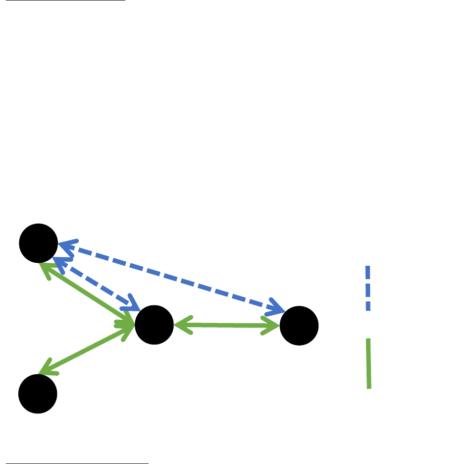
a hub, change planes, and reach their final destination via a connecting flight. Consider the

simple system in Figure 2 with airports P, Q, R, and hubbed airport H. Suppose that a passenger

wants to travel from airport P to airport R. A point-to-point network (dashed lines) would allow

Load factor is a measure of capacity utilization. It is the proportion of total seats available that are filled by

passengers. Often it is calculated by dividing the total available seat miles by the total number of passenger miles.

Point-to-point

Hub-and-spoke

Figure 2. A simple diagram of a hypothetical hub-and-spoke network (solid lines) versus a point-to-point network

(dashed lines) connecting four airports. In a hub-and spoke system, airport H represents the hub airport.

them to fly directly to R without any connections. Only passengers traveling from P to R would

be on this flight. Alternatively, with a hub-and-spoke network (solid lines), a passenger would

have to make a connection at hub H, which may be less convenient and will take longer.

However, say that the passenger wanted to travel from Q to R. This may not be an option in a

point-to-point system where demand is insufficient, but, in a hub-and-spoke network, a

passenger may fly from airport Q to hub H, where the hub airline can collect demand from

airports P, Q, and H to fly from hub H to airport R. The airline benefits from economies of scale

as is can fly bigger planes that have more capacity filled, and fly routes with higher frequency.

Also, the hubbed airport, airport H, now has direct flights (from its perspective) to three different

locations. In the point-to-point model, H may just have had service to P. However, concentrating

traffic at hub H could lead to congestion and higher airfares from increased airline market power.

If the dominant airline were to de-hub H, possibly other carriers, such as low-cost carriers, could

enter and put downward pressure on airfares.

In summary, when an airline employs a hub-and-spoke network, it has both positive and

negative implications for consumers. The increased scale may mean better services, facilities,

and choice. Flight frequency and options should increase greatly. These networks also mean that

carriers are better able to serve longer routes while filling the capacity of their planes, and

offering more connections, generating more competition on longer routes. The choice of

departure times has also vastly grown since deregulation and with the rise of hub-and-spoke.

Consequences of hub-and-spoke are congestion and the inconvenience of having to change

planes and even airlines. Congestion can lead to issues like missing a connection due to delay or

losing luggage (Borenstein, 1992). Fageda and Flores-Fillol (2015) suggest in their welfare

analysis that in hub-and-spoke networks, airlines are biased towards inefficiently excessive flight

frequencies leading to airport congestion.

Airlines derive cost and competitive advantage from hub-and-spoke networks. There tend

to be many more route options for passengers that could not be practically served by a nonstop

flight where demand would be insufficient or prices too high. Economies of density, where

airlines can increase flight frequency and fill planes up to higher load factors, are obtained on the

cost side thereby reducing cost per passenger (Brueckner, Dyer, & Spiller, 1992). Airlines may

also exploit economies of scale and scope at a hub airport. Because airlines can funnel people

from multiple origins onto a single route, larger planes are used which tend to have lower costs

per passenger. This effect may not offset the increased distance that an airline must fly a

passenger. Carriers also benefit from synergies of a concentrated and localized operation; a hub

provides an airline a central place to complete aircraft maintenance, and labor may be used more

effectively (Aguirregabiria & Ho, 2012). Most airports can only act as a hub for a single airline

due to logistic and capacity restraints, leading to airport dominance and substantial effects on

carrier concentrations, so market power is often an issue at hubs (Borenstein & Rose, 2014).

What hub-and-spoke networks offer in cost savings may be taken away given the market

power they afford. Airport capacity constraints may also drive inefficiencies. Sinclair (1995)

found empirical evidence that hub systems deter entry and encourage the exit of rivals. This is

beneficial if a prospective entrant is a higher-cost firm, but detrimental otherwise (Sinclair,

1995). Furthermore, Hendricks et al. (1997) conclude that hub operators can pose a credible

threat to competitors and entrants on spoke route markets where a hub airline may be willing to

continue operating a route while suffering losses to encourage the exit of rivals (Hendricks,

Piccione, & Tan, 1997). Aguirregabiria and Ho (2012) find similar evidence consistent with hub

airlines deterring competition in markets on spoke routes.

Airfare

In the literature there exists the idea of a “hub premium.” A hub premium is often

attributed to the market power of the hub airline, where flights to and from a hub airport are

relatively more expensive than an equivalent non-hub flight. Borenstein (1989) found evidence

of increased efficiency in the use of aircraft in hub-and-spoke systems compared to point-to-

point models, but that airport dominance by just a single carrier from hub formation resulted in

higher fares for passengers traveling to or from those airports – passengers that were not using

the hub airport as a connection. He suggests there are cost savings that are not passed along to

consumers, though travelers may benefit from more flights and convenient connections out of

their home airport. Despite higher prices on some airlines, loyalty programs deter passengers

from searching for the minimum fare. The benefit to a dominating carrier of inflated airfares

does not transfer over to competitors on the same route (Borenstein, 1989).

According to Brueckner, Lee, and Singer (2013), it has been well established that

airlines’ market fares do respond to the level of competition. However, there has been a low-cost

carrier revolution, most notably with Southwest Airlines, putting downward pressure on prices

for domestic flights. In their study, Brueckner et al. (2013) consider competition from adjacent

airports and take a novel approach by considering both legacy and low-cost carriers. They find a

much higher impact in prices from Southwest and other low-cost carries compared to introducing

competition from another legacy carrier onto a route (up to 26% lower airfares when Southwest

enters a nonstop market). However, while still significant, the effect of low-cost carriers reducing

prices is diminished in connecting versus nonstop markets (Brueckner et al., 2013). With freed

up airport capacity following a legacy carrier de-hubbing, there is potential for a low-cost carrier

to enter or expand operations, lowering fares.

Quality

Attempting to quantify service like in-flight experience is very difficult, but there is

abundant data on flight delays. One obvious reason for delays comes from severe weather, but

delays also stem from airport congestion – limited increases in capacity and fewer investments in

infrastructure than necessary to keep pace with demand (Borenstein & Rose, 2014). We can

quantify flight delay outcomes with on-time performance data for carriers. If an airport saw its

capacity diminish significantly, through de-hubbing or another event, we might expect fewer

delays.

Israel, Keating, Rubinfeld, and Willig (2013) develop another way of incorporating

quality effects into consumer welfare considerations at hub airports, finding that improvements

in quality overcome the higher fares at hub airports, possibly yielding more consumer welfare

than non-hub airports. They advocate for the benefits of network effects in improving

connectivity and schedules. Borenstein and Rose (2014) acknowledge the benefits of a hub for

local demand because of the disproportionate number of flights available compared to what

would otherwise be offered (Borenstein & Rose, 2014). Furthermore, Israel et al. (2013) cite

continuing work by Borenstein that finds nominal hub premiums have fallen since the 1990s

with the rise of low-cost carriers and improved costs. Israel et al. (2013) determined a nominal

fare premium during 2009 and 2010 of 17.6% for CLE. The authors then computed a quality-

adjusted airfare, finding that CLE had a calculated negative hub premium of -8.2%. There was a

similar trend at other hub airports. While the level of quality adjustment used by Israel et al.

(2013) is outside the scope of my research, I will account for quality by identifying any changes

in on-time performance, flight frequency, and destinations offered at CLE.

Mergers

After deregulation, there was a wave of new entrants followed by a large number of

mergers. Stricter antitrust policy driven by concerns for competition and hub dominance meant

that by 1990, mergers were less frequent. Other partnerships formed between small regional

airlines and national carriers, allowing for more schedules to sync up, especially at hubs,

increasing value for passengers and airlines alike. The relationship is symbiotic where regional

airlines feed into a hub. With the financial crisis, we then saw a flurry of mergers following 2008

(Borenstein & Rose, 2014). Borenstein and Rose (2014) question whether policymakers should

see market power generated from mergers and hub-and-spoke networks as a threat to consumers

and smaller competition. In an industry where capital and operating costs are high, and earnings

are low, is antitrust policy still necessary? One could argue that barriers to entry and the market

power seen at hub-and-spoke airports lead to deadweight loss by allowing the dominant airline to

survive and retain market share rather than being ousted by a collection of more efficient rivals.

Given this efficiency argument, de-hubbing should benefit the smaller, more efficient airlines

who have cost advantages. Less market power could lead to lower airfares and more competition,

resulting in a faster recovery of flight capacity at de-hubbed airports like CLE.

De-hubbing

The choice to de-hub is part of the effort to find the optimal level of hubs in a hub-and-

spoke network. With the freedom to choose routes, price routes, and merge with rivals, an

airline’s choice to de-hub is a full network question, for which I study the effects at CLE. In their

theoretical paper, Bilotkach, Fageda, and Flores-Fillol (2013) study network reorganization of

hub-and-spoke networks following mergers. After consolidation, an airline may divert traffic

from a primary hub to a secondary hub to alleviate congestion. However, in a model without

congestion, the airline may prioritize its primary hub (Bilotkach et al., 2013). While Bilotkach et

al. (2013) recognize caveats in their theoretical model, we could assume that following its

merger with Continental, United decided to prioritize its hubs in Chicago and Newark rather than

CLE. More signals that too many hubs are suboptimal come from Wojahn’s (2001) theoretical

model. Under economies of density, which can be thought of as economies of scale along a

route, Wojahn defines a cost-minimizing network as one that combines point-to-point operations

with a single hub. Costs increase when an airline routes passengers between endpoint airports via

more than one hub (Wojahn, 2001).

Luo (2014) studied airline network structure change and consumer welfare through the

lens of mergers. When legacy carriers merge, such as United and Continental, they both bring

their respective hub-and-spoke network operations together. When there are overlaps and

redundancies in the combined networks, the merged airline looks to reduce costs and benefit

from synergies by reorganizing traffic and hubs in their network. Following a merger, smaller

hubs or ones with weak demand are candidates for de-hubbing. Delta downsized operations at

Cincinnati after merging with Northwest because of acquired hubs nearby, and an economic

impact report from Northern Kentucky University found far-reaching effects on jobs, output, and

tax revenues (Luo, 2014). Luo finds that consumer welfare increased at Cincinnati, despite the

loss of direct service to many airports, because the removal of the hub premium substantially

reduced fares, at least in the short-run.

Tan and Samuel (2016) study the effect on average airfares following de-hubbing at

seven different airports between 1993 and 2009. They empirically confirm what theory might

suggest: whether airfare on direct flights at hub markets significantly increased or decreased was

driven by the entry or presence of low-cost carriers who put downward pressure on airfares (Tan

& Samuel, 2016). Low-cost carriers exploited the gap in the market and increased flight

frequency and the number of routes in some de-hubbed airport cases. If they did not, average

airfares rose. Outside of the U.S., the de-hubbing of Budapest by Malev Hungarian Airlines led

to net decreases in airport capacity where decreased frequency may have offset the lower airfares

associated with low-cost carriers increasing capacity (Bilotkach, Mueller, & Németh, 2014).

Redondi, Malighetti, and Paleari (2012) identify and study examples of de-hubbing worldwide.

In their cases, significant decreases in departures and available seats persisted after the de-

hubbing event, so airports did not fully recover to hub-level traffic. However, the number of

destinations served was reduced relatively less (Redondi et al., 2012). Airports tended to

experience faster recoveries when low-cost carriers replaced some hub carrier traffic (Redondi et

al., 2012). While Redondi et al. (2012) did consider airports in the U.S., airports in other

countries may face very different circumstances, possibly even competition from other modes of

transport such as rail. Rupp and Tan (2016) similarly find the expected significant decrease in

flight frequency and nonstop destinations offered, but stress the benefits of airports no longer

suffering from congestion. Passengers benefit from fewer delays, fewer cancelations, and shorter

travel times. They conclude that reliability of the de-hubbing airline and competitors improves in

the majority of the four cases studied (Rupp & Tan, 2016).

My research contributes to the de-hubbing literature with in-depth empirical analysis and

results that focus on airfare and quality impacts of CLE losing its hub status. I uncover de-

hubbing driven effects on CLE passengers from changes in airfare per mile, seat capacity, the

frequency of flights, number of destinations served, delays, and market structure. I also explore

the recovery patterns at CLE as rival carriers make strategic responses to United’s decision.

IV. Data

I construct my datasets from several U.S. Department of Transportation Bureau of

Transportation Statistics (BTS) data sources and metropolitan statistical area (MSA) information

from the U.S. Department of Commerce’s Bureau of Economic Analysis (BEA).

DB1B: Airline Origin and Destination Survey

My source for passenger airfare information is the Airline Origin and Destination Survey

(DB1B), a quarterly 10% sample of all domestic airline itineraries from carriers that report to the

BTS Office of Airline Information. The DB1B database is split into three data tables – Coupon,

Market, and Ticket (itinerary) – that may be merged. An itinerary describes a whole trip which is

often composed of multiple flights and connections. Coupons represent each flight segment in an

itinerary. Each time there is a change of plane there is a new coupon, so in a sense, a coupon may

be thought of like a boarding pass. DB1B splits itineraries into a market based on trip breaks. If a

passenger stops at the destination of a ticket coupon to engage in any activity other than using

the airport as a connection and changing planes, then the stop is designated as a trip break. The

coupons on either side of the trip break become part of a market. We can understand this through

the example in Figure 3 of visiting Los Angeles from Boston via a connection in Cleveland. The

itinerary would contain information on the passenger’s travel from Boston. It has information on

absolute origin, final destination, and a roundtrip indicator. Each coupon is part of an itinerary

1 Itinerary 4 Coupons 2 Markets

BOS to LAX, roundtrip BOS:CLE BOS to LAX

(BOS:CLE:LAX:CLE:BOS) CLE:LAX LAX to BOS

LAX:CLE

CLE:BOS

Figure 3. An example of how itineraries relate to coupons and markets in the Airline Origin and Destination

Survey. This hypothetical passenger travels roundtrip from Boston to LA via Cleveland.

and represents one of the four flight segments, or legs, between BOS, CLE, and LAX that make

up the trip. Lastly, since the passenger is visiting LA, we know that a trip break exists, which

splits the itinerary into two separate markets, one for each direction of travel. Direct flights

would be made up of a single nonstop market and single coupon.

Note that there are also two types of carrier identified in DB1B: ticketing carrier and

operating carrier. The ticketing carrier is whom a passenger buys the ticket from, the airline that

shows up on an itinerary or boarding pass, and the name seen on the tail of the plane. The

operating carrier is the airline that actually runs the flight, owns the equipment, and employs the

crew. In many cases, the ticketing and operating carriers are not the same, especially on regional

flights which national carriers tend to brand but not operate. For example, a United Express

flight ticketed by United Airlines could be operated by Republic Airline. For most of my

analyses, I consider operating carrier because each operating carrier has a unique cost structure

that is lost when subsetting by ticketing carrier. A single route may be operated by multiple

operating carriers under the umbrella of a single ticketing carrier. The only time I use ticketing

carrier in my analyses is when calculating market concentration measures because it is the

ticketing carriers that directly compete with one another.

In the DB1B dataset, I restrict my analyses to origin-destination passengers in nonstop

directional markets. A nonstop market is a one-way itinerary (route) consisting of one coupon

(one flight segment) or a roundtrip itinerary that is broken up into one nonstop flight for each

direction. An origin-destination passenger is a traveler who originates from one route endpoint,

say airport A, in the market, and the other route endpoint, say airport B, is their destination.

Origin-destination passengers share nonstop markets with connecting passengers. A connecting

passenger could originate from airport A to catch a connecting flight at airport B, in order to

reach their final destination at airport C.

There are practical and theoretical reasons for deciding to consider origin-destination

passengers on nonstop flights. For itineraries with connections, an airfare is only provided for the

whole itinerary, not for each coupon. One airfare across multiple flight segments on an itinerary

does not allow me to disentangle the specific flight segment effects because a passenger will

encounter routes with different characteristics since their travel will include more than one

airport pair, which may be serviced by more than one operating or ticketing carrier. Imputing an

airfare for a flight that is one portion of a longer trip would miss these effects and dilute them

across the other imputed airfares on the full route. My focus is not on estimating the network

effects of de-hubbing. If it were, then connecting flights would be relevant. Instead, I use the

action of de-hubbing by United as an event study for CLE, and to understand the effects on

passengers departing from CLE, not necessarily using CLE as a hub. Furthermore, prices paid by

origin-destination passengers in nonstop markets may act as a proxy for the airfare faced by

connecting passengers using the nonstop market as one of their connections. According to

Brueckner et al. (2013), connecting passengers in nonstop markets tend to be dominated by

origin-destination passengers on the same flight who compose a larger proportion of the total

travelers. Constructing my nonstop market DB1B dataset retains a majority of the passengers

captured in the DB1B survey.

To ensure that my airfare analysis is reliable, I only consider coach class fares, which

constitute around 90% of the fares paid by passengers in the sample. I keep routes where both

endpoint airports are one of the 110 largest airports based on enplanement;

this includes CLE.

Data and rankings from the Federal Aviation Administration for total passenger boarding at all commercial service

airport during the 2014 calendar year. CLE was ranked 47.

To exclude anomalous airfares, I require that an airfare is at least $25,

but less than a rate of $3

per mile flown,

airfares outside these bounds may be part of a loyalty program, a higher-class

ticket, or a coding error. Additionally, I utilize a credibility flag provided by BTS to omit airfares

deemed questionable based on credible limits. Finally, I drop bulk fares which are rare in the

data but do not represent the actual value of the airfare.

With the three DB1B tables combined, each observation is the common airfare paid by a

certain number of passengers to travel with a given operating carrier in a specific nonstop

market, along with other route characteristics. Passengers will pay different airfares on the same

route with the same carrier at different times in a quarter, and also different amounts on a single

flight. Thus, there are not unique observations for each carrier-route-quarter group. Therefore, I

aggregate DB1B by operating carrier,

route, and year-quarter, such that each observation

provides information on passenger-weighted mean airfare

and mean airfare-per-mile for a

carrier-route in the quarter; origin and destination airports; operating carrier; and ticketing

carrier.

T-100: Air Carrier Statistics

For quantity and capacity information, I use the BTS Air Carrier Statistics T-100 data

bank (T-100). T-100 is not a sample. It provides total values for all reporting carriers and is

The minimum cutoff is consistent with past literature, see Brueckner et al. (2013),

This maximum bound follows BTS publications standards.

DB1B is aggregated by operating carrier rather than ticketing carrier because multiple operating carriers may be

used by a single ticketing carrier, and so that DB1B may be merged with T-100 which only reports operating carrier.

If two airlines merge within my sample, all flights prior to the two airlines jointly reporting are attributed to the

single airline code that exists following the merger. BTS provides the following information which I account for in

my sample: Continental Micronesia (CS) was combined into Continental Airlines (CO) in December 2010 and joint

reporting began in January 2011. Atlantic Southeast (XE) and ExpressJet (EV) began reporting jointly in January

2012. United (UA) and Continental (CO) began reporting jointly in January 2012 following their 2010 merger

announcement. Southwest (WN) and AirTran (FL) began reporting jointly in January 2015 following their 2011

merger announcement. American (AA) and US Airways (US) began reporting jointly as AA in July 2015 following

their 2013 merger announcement.

Itinerary fares are not adjusted for inflation.

reported monthly. I rely on the T-100 Domestic Segment dataset, which is analogous to the

coupon level information in DB1B. T-100 provides total values for flights by operating carrier,

irrespective of what the starting origin or final destination is for a passenger (on their itinerary).

Therefore, T-100 captures all passengers on a flight segment, both origin-destination, and

connecting passengers. In my T-100 sample, I require an airline carrier to transport at least 400

passengers, and complete 13 or more departures on a route in the quarter to retain the

observation in my sample. Applying these constraints removes passenger markets that are too

small. I do not make any passenger-type restrictions to T-100 as I do for airfares in DB1B as

there are no equivalent theoretical or practical concerns. T-100 origin and destination pairs are

restricted to the same 110 airports as DB1B. Each T-100 observation has information on the total

number of passengers transported, available capacity (total number of seats offered), and the

total number of departures performed by an operating carrier on a given route in a given quarter.

Route characteristics like origin, destination, distance flown, and aircraft type,

are also included.

DB1B, T-100, MSA Dataset

For T-100 and DB1B, I have 28 quarters of observations, from 2010Q1 through 2016Q4.

Given that United’s de-hubbing of CLE occurred in 2014, this provides an informative number

of quarterly observations both before and after de-hubbing. To combine the airfare information

from DB1B and the quantity information in T-100, I merge the datasets on operating carrier,

origin, destination, year, and quarter. The final dataset is still at the carrier-route-quarter level.

also identify airports’ host MSAs and attach yearly observations of origin and destination MSA

populations and per capita incomes to the merged (T-100-DB1B) dataset. Across 28 quarters of

Aircraft type is based on the type of aircraft used most frequently by the operating carrier on the route in the

quarter.

97% of T100 observations successfully match to a DB1B counterpart. Non-matches tend to be smaller flights on

more obscure carriers.

data, I have 194,654 observations. There are 38 operating carriers, 18 ticketing carriers, 110

origins and destinations, and 4,241 routes. Table 1 presents summary statistics for the dataset.

The mean airfare is $210.98, corresponding to a mean airfare per mile of 41 cents. Total seats

offered quarterly on carrier-routes averages to almost 25,000 seats across 216 departures. Figure

4 is discussed later and provides an improved picture of CLE and other airports before and after

de-hubbing.

On-Time Performance Dataset

From BTS, I also incorporate the On-Time Performance data table. I aggregate these data

at the operating carrier-route-quarter level for information on average delays, and the fraction of

flights that are delayed by 15 minutes or more. For analysis, I merge these variables onto my T-

100 and DB1B datasets. There are 30% fewer observations because on-time performance is only

reported for major carriers,

not all the carriers that I consider in my other analyses. The result is

131,058 observations across 28 quarters. In Table 1 we see that, on average, 18% of departures

are delayed by 15 minutes or more, and the mean delay for departures is 10 minutes.

Airport Level Dataset

For analyses that I conduct at the airport level, I construct a final dataset that aggregates

data from DB1B and T-100 by origin airport and quarter. Average airfare and distance are

weighted by the total number of passengers out of the origin airport. Total numbers of

passengers, seats,

and departures are all summed up by quarter from constituent operating

carriers along all routes. Mean distance is weighted by total number of seats. Origin airport MSA

population and per capita income are retained. In addition, from T-100 data in the aggregation

process, I calculate market structure metrics for origin airports in my sample, including

BTS considers a carrier to be a “major carrier” if it has annual revenues that exceed $1 billion.

Number of passengers and seats departing from the origin airport.

N Mean SD Minimum 1st Quartile Median 3rd Quartile Maximum

DB1B, T-100, MSA data (carrier-route-

qaurter level):

Airfare ($) 194,654 210.98 71.26 25.00 159.39 207.15 258.50 733.74

Airfare per mile ($/mi) 194,654 0.41 0.32 0.02 0.19 0.31 0.50 2.99

Total passengers 194,654 20,291 27,084 400 4,242 10,447 23,889 270,216

Total seats 194,654 24,949 32,470 481 5,450 12,882 29,390 292,506

Total departures 194,654 216 216 13 77 153 272 2,284

Distance, miles flown (mi) 194,654 777 524 55 395 642 1,012 2,724

Per capita income, Origin ($) 194,654 48,291 8,789 28,074 42,168 46,679 53,360 87,643

Per capita income, Destination ($) 194,654 48,291 8,789 28,074 42,173 46,679 53,360 87,643

Population, Origin 194,654 4,761,904 4,877,396 83,459 1,572,482 2,828,665 6,001,717 20,153,634

Population, Destination 194,654 4,768,710 4,891,979 83,459 1,570,802 2,828,665 6,001,717 20,153,634

On-time performance (carrier-route-

qaurter level):

Fraction of departures delayed >15 mins 131,058 0.18 0.09 0.00 0.12 0.17 0.24 0.95

Average departure delay (mins) 131,058 10 8 -12 4 9 13 223

Airport level data (origin airport-quarter

level):

Average airfare ($) 3,080 197.18 37.55 64.45 176.95 198.27 221.75 321.93

Average airfare per mile ($/mi) 3,080 0.42 0.16 0.08 0.31 0.40 0.51 1.27

Total passengers 3,080 1,282,366 1,639,134 14,099 210,184 519,372 1,787,591 10,620,810

Total seats 3,080 1,576,734 1,965,603 16,050 265,958 656,662 2,168,674 12,150,914

Total departures 3,080 13,631 15,627 107 3,533 6,396 17,401 86,063

Avearge seats per flight 3,080 104 28 51 81 103 125 207

Average distance (mi) 3,080 681 221 321 512 647 805 1,577

HHI 3,080 0.39 0.19 0.17 0.27 0.32 0.43 1.00

Top carrier market share 3,080 0.51 0.19 0.23 0.36 0.45 0.60 1.00

Number of operating carriers 3,080 12 5 1 9 12 16 24

Number of ticketing carrier 3,080 5 2 1 4 5 6 12

Number of destinations served 3,080 31 23 2 13 21 47 96

Summary statistics for three datasets for analyses covering 2010Q1 through 2016Q4.

Note: Table 1 reports the number of observations, mean, standard deviation, minimum, first quartile, median, third quartile,

and maximum for relevant

variables. Observations in the DB1B, T

-100, MSA dataset and in the on

-time performance dataset are at the carrier

-route quarter level. Observations for

the airport level data are at the origin airport

-quarter level.

Table

Summary statistics for the three datasets I consider for analyses.

Herfindahl-Hirschman Indexes based on departing seat market share of ticketing carriers;

one-firm concentration ratio (CR1) for the market share of seats held by the largest dominant

ticketing carrier; number of operating and ticketing carriers; number of unique destinations

offered; and average plane size in terms of seats per flight. Across 28 quarters and 110 airports, I

have 3,080 observations in the airport level dataset. The descriptive statistics in Table 1 are

averaged by airport and indicate that the average airport airfare is $197.18 and average airfare

per mile is 42 cents. The average airport has 13,631 departures, transporting almost 1.28 million

passengers per quarter by providing 1.58 million seats. The mean airport HHI across the 110

airports over 28 quarters is 0.39 with 12 operating carriers and 5 ticketing carriers present. 31

unique destinations are served at the average airport, and the mean distance flown out of airports

is 681 miles.

The De-Hubbing of Cleveland by United Airlines in the Data

Figures 4 (a) through 4 (f) compare characteristics of CLE to “Others,” the 109 other

airports in my sample, pre- and post-de-hubbing. In all cases, values for CLE and “Others” are

normalized to 100 in 2010Q1 for a clear comparison of pre-de-hubbing trends. Data are quarterly

at the origin airport level. The two vertical dashed lines represent the period United was de-

hubbing CLE, starting when the decision was purportedly made, and ending when the de-

hubbing was scheduled to for completion. Generally, before de-hubbing, measures at CLE move

with the rest of the sample. Figure 4 (a) shows normalized airfare per mile over time for the

average departing flight,

we see a clear drop for CLE relative to other airports, lagging the de-

hubbing event by a few quarters. Figures 4 (b) and (c) show the capacity changes at CLE

HHI formula for quarterly market share calculations for each of the top 100 airports:  











where 





 is airline i's market share of seat capacity at airport j in quarter q.

Airfare per mile is weighted by number of passengers for “Others” quarterly calculation.

100

110

120

130

Airfare per mile (normalized)

2010 2011 2012 2013 2014 2015 2016

CLE Others

CLE compared to other airports, 2010Q1 - 2016Q4.

Airfare Per Mile

100

110

120

Total seats (normalized)

2010 2011 2012 2013 2014 2015 2016

CLE Others

CLE compared to other airports, 2010Q1 - 2016Q4.

Total Seats

100

110

Total departures (normalized)

2010 2011 2012 2013 2014 2015 2016

CLE Others

CLE compared to other airports, 2010Q1 - 2016Q4.

Total Departures

100

HHI (normalized)

2010 2011 2012 2013 2014 2015 2016

CLE Others

CLE compared to other airports, 2010Q1 - 2016Q4.

Airport HHI

100

110

Number of destinations (normalized)

2010 2011 2012 2013 2014 2015 2016

CLE Others

CLE compared to other airports, 2010Q1 - 2016Q4.

Number of Destinations Offered From Airport

100

150

200

250

300

Fraction (normalized)

2010 2011 2012 2013 2014 2015 2016

CLE Others

CLE compared to other airports, 2010Q1 - 2016Q4.

Fraction of Departures Delayed >15mins

(d)

(b)

(c)

(e)

(f)

(a)

Figure 4. Airport level time series graphs comparing CLE (solid blue line) to the other 109 airports (dashed red

line) in my sample. Values are plotted quarterly from 2010Q1 through 2016Q4 and normalized to 100 in

2010Q1. The vertical dashed lines represent the period during which de-hubbing was purportedly announced,

carried out, and completed. (a) Mean airfare per mile weighted by number of passengers. (b) Total seats

departing CLE and sum across other airport total seats. (c) Total departures from CLE and sum across other

airport total departures. (d) CLE HHI and mean of HHI’s across other airports. (e) Number of destinations

offered from CLE and mean number of destinations from other airports. (f) Fraction of departures delayed more

than 15 minutes out of CLE and average fraction of delays at other airports.

following de-hubbing for normalized total seats and normalized total departures, relative to the

normalized sum of totals across the 109 other airports. There appears to be a recovery in quantity

of seats at CLE during 2015 and 2016. We also see this trend for the total of seats at other

airports. A roughly 30% or 40% reduction in departures does not appear to rebound. The path of

HHI at CLE in Figure 4 (d) demonstrates changes in market structure as United Airlines removes

itself from the dominant carrier position. A quality measure, number of unique destinations

offered, looks to be a victim of de-hubbing in CLE, falling 40% in Figure 4 (e). There is no clear

trend in delays following de-hubbing in CLE in Figure 4 (f). Figure 4 motivates why a

difference-in-differences method should be an appropriate approach to identify significant

changes and test causality. Before de-hubbing, trends across all airports and CLE were similar.

Then, during and after de-hubbing, we can compare changes at CLE to changes in the control

group of airports over time.

V. Econometric Approach

I use a difference-in-differences (DID) approach to identify causal relationships between

the de-hubbing of CLE by United and various outcomes that are important to passengers. The

impacts on passengers departing from CLE that I test for include changes in airfare, market

structure, quality measures such as frequency of flights and delays, and seat capacity. I perform

these analyses on all carriers and routes in my sample across all 110 airports for observations

from 2010Q1 through 2016Q4.

Carrier-Route-Quarter Level Econometric Model

The primary response variable I consider is the natural log transformed mean airfare per

mile. Here my observational unit is carrier-route by quarter. I control for distance flown as a

cubic

and endpoint MSA airport characteristics. I also include extensive fixed effects as

detailed in the specification below. I construct the DID interaction terms of interest from a

dummy variable for CLE as an origin airport – the treatment group – and dummy variables for

time periods surrounding and including de-hubbing. The corresponding main effect binary

variable for CLE is absorbed by the origin fixed effects, and the dummy variables indicating the

time periods preceding, during, and following de-hubbing are absorbed in the year-quarter fixed

effects. Accordingly, the specification for my difference-in-differences model is given by:











 



 







  



  







  





 













 















 















 







 





 







 





 







 





 







 





 



 



 



 



 



 





where airfarePerMile

irq

is the mean airfare per mile to travel with carrier i, on route r, during

year-quarter q; 



is a constant; CLE

is an indicator variable for if Cleveland airport is the origin

on route r; post.dehub

is an indicator variable for if the period q is after de-hubbing, 2014Q3

and onwards; during.dehub

indicates if the period q is during the de-hubbing announcement and

process period, 2014Q1 and 2014Q2, this way I do not need to omit data from those two quarters

from my analyses, and it does not interfere with the pre-dehubbing baseline period; distance

the miles flown on route r; pop.origin

, pop.dest

, inc.origin

, and inc.dest

are the respective

populations and per capita incomes of the endpoint airport MSAs on route r for the year covering

year-quarter q; 



represents year-quarter fixed effects, from 2010Q1 through

The distance of a flight has price effects moving in different directions. Longer flights tend to be more expensive,

while in terms of airfare per mile they may be cheaper since the costs are spread among more passengers with no

more time spent organizing on the ground.The change is airfare may also be different depending on the proportional

increase in miles flown.

2016Q4, to account for seasonal variation and network-wide changes over time; 



and





are origin airport and destination airport fixed effects, respectively, included to cover

endpoint airport characteristics I cannot capture elsewhere; operating carrier fixed effects, held in





, capture differences in operating costs and the type of carrier, whether it be a low-cost,

legacy, or regional carrier; aircraft group fixed effects are given by 



, which consider

the type of airplane such as turbo prop versus jet, and the number of engines, to further capture

operating costs; and 



is the error term. Standard errors are clustered by route to compensate

for within-route correlation over time.

The primary coefficient of interest in the above specification is the DID estimator 

which identifies the change in airfare per mile for CLE departures that we can attribute to the

post-de-hubbed period relative to the pre-de-hubbed period and the control group. In my

analyses, I update the DID specification such that the treatment and time period interaction terms

are biannual or quarterly. I interact CLE

with indicators for 2010H1 through 2016H2

respectively, omitting the CLE

interaction with  



for a base quarter, giving:











 



 







  



  







  



  

 







  



  







  



  

 







  



  













 















 















 







 





 







 





 







 





 







 





 



 



 



 



 



 





where  



indicates that the half-year corresponds to year-quarter q. Recall that plans to

de-hub were revealed in 2014Q1, and de-hubbing was to finish by the end of 2014Q2. Therefore,

the coefficients of interest for effects caused by de-hubbing become the DID estimators for

This approach is consistent with previous literature, including Brueckner et al. (2013).





  



 and onwards. Incorporating DID interactions based on half-year, I can

form a better understanding of immediate effects caused by de-hubbing, any lagged effects, and

the recovery pattern that follows. I can also verify that my response variable was relatively stable

during the period preceding de-hubbing. A negative coefficient estimate that is statistically

significant for interaction terms in periods during and after 2014H2 indicate that ticket prices, as

measured by mean airfare per mile, fell due to United’s decision. Likewise, we can consider

coefficients for interactions with the treatment group during 2014H1 to detect effects during de-

hubbing. These DID estimators will also be useful when looking at other responses, such as

quantity measures during United’s changes. Quartlery, rather than biannual, interactions with

CLE

are implemented analogously, omitting the i.2013Q4

(indicator for fourth quarter of 2013)

interaction for a baseline instead.

This specification is effective because it can explain a large proportion of the variability

in prices while not relying on explanatory variables that are outcomes of de-hubbing, variables

which would suffer from endogeneity – quantity and market structure metrics, for example.

Assuming that the parallel trends assumption holds, which is supported by visual inspection of

pre-de-hubbing movements presented in Figure 4, using a difference-in-differences approach

allows me to make a causal inference. Having a large 109 airport control group across 28

quarters ensures that my DID does not identify effects in the treatment group – flights originating

from CLE – felt elsewhere in the airline network that were unrelated to the de-hubbing.

Potential Limitations

My identification strategy is potentially limited by the variables I can include in my

regression specification. Endogeneity of variables in my regression model was a potential

concern, and the variables I have included are chosen carefully to avoid this issue.

Available

traditional predictors of price, such as number of seats and number of departures, which capture

supply, are clear outcomes of de-hubbing, which is a reduction in capacity, making them

endogenous. Market structure measures like HHI are also afflicted and suffer from simultaneity

bias. As United is de-hubbing, the HHI at CLE is expected to change. Even with United omitted

from the CLE HHI calculations, this would not account for responses to de-hubbing from other

carriers.

As addressed in Tan and Samuel (2016), lower airfares could present a reverse causality

issue in that downward pressure on airfares from rivals could have decreased airfares at CLE and

provoked United to de-hub. We know that according to United’s CEO, the airline was losing

money at the CLE hub for over a decade, but it is not explained why. There is a low-cost carrier

presence in CLE before 2014; however, we do not see much variability in prices, and it is more

likely that the de-hubbing was motivated by the recent merger between United and Continental,

rather than airfare price competition on routes that United dominated. As discussed in Figure 6,

we also see that airline rivals and low-cost competitors do not appear to expand capacity until

after United de-hubs. No literature attributes the de-hubbing for CLE to low-cost carriers, and

Tan and Samuel (2016) do not find this phenomenon to be the case in any of the seven de-

hubbings they encounter.

A general limitation in any study of a single airport is how all airports are tied together in

a network. Airlines form hub-and-spoke or point-to-point networks across the United States, so

every decision in the system may have effects multiple levels away in the network. Network

effects pose challenges for identifying impacts of de-hubbing in CLE because so many other

I deemed an instrumental variable approach inferior to the model I settled on because there are no instruments

I am comfortable with that are not related to price.

actions and changes are happening simultaneously across the network. To mitigate this concern,

I include in my sample the 110 largest airports in the United States and use the 109 airports that

are not CLE as a control group. I think that selecting one or a small group of control airports

could pose more serious issues than potential issues with my large control group. I believe that

my strategy reduces the chance of having other large events disturb my understanding of the de-

hubbing effects in the difference-in-differences model because, relative to the nationwide

network, changes at individual airports are less consequential and outweighed by relative

stability elsewhere. I am still able to capture system-level shocks, trends in airfare, and changes

in other relevant responses. Having an appropriate control group is essential for presenting a

causality argument. As a robustness check for the suitability of the control airports for CLE, I

form subsamples of my dataset based on similarity of endpoint airports to CLE. The results are

provided in Table 3.

Additional Tests

In addition to testing for the impact on airfare per mile from de-hubbing CLE, I apply my

difference-in-differences model to analyze other response variables. I consider changes in

quantity and capacity at the carrier-route level by quarter using the natural logged total number

of seats offered and natural logged total number of departures as responses. Number of

departures can also be considered a quality measure because a higher frequency of flights is

often more convenient for passengers. Another measure of quality is the on-time performance of

flights. I run the same regression on the fraction of departures that are delayed by at least 15

minutes, and on the natural logged mean delay in minutes for departures. For all these dependent

variables, the right-hand-side of the specification remains unchanged from my initial

specification for airfare per mile since the covariates and fixed effects are not specific to price

and should explain a reasonable amount of the variation in these new responses. Corresponding

to the DID for natural logged airfare per mile, the coefficients of interest and statistical tests are

identical.

Identifying a relationship between de-hubbing and departure delays has unique

limitations. Because weather and mechanical issues, not just airport congestion, cause delays

(which can propagate throughout a carrier’s network), the data, and any relationship, are much

more noisy. We can see this in the lack of a clear pattern in Figure 4 (f). De-hubbing could lead

to less congestion and fewer delays; alternatively, if rivals enter or expand operations out of CLE

in response to United’s de-hubbing, then delays could increase because coordination across more

players is harder. Ability to detect a change could potentially be improved in my model by

including weather information across the United States and a better idea of network effects. This

would be a laborious process that also faces challenges. Given that the scope of my research is

broader than the response of delays to de-hubbing, I use the same regression specification as for

other dependent variables.

Airport Level Econometric Model

I also approach the analysis of de-hubbing impacts from the airport level. As described in

the data section, I aggregate the carrier-route-quarter level dataset into the origin airport level

such that my observational unit is airport by quarter. The airport level dataset also covers the

full-time period from 2010Q1 through 2016Q4.

At the airport level, I look for the causal relationship between de-hubbing and capacity,

market structure, and quality outcomes. The capacity and quantity response variables I consider

are total departures, total seats available, and the average plane size across quarters at each

airport – all are natural log transformed. Total seats is a measure of overall capacity, and with

departures, the coefficient estimates will demonstrate that United’s de-hubbing had a statistically

significant effect on CLE as a whole. Departure frequency and average plane size are quality

measures in terms of convenience and comfort, and larger planes may also indicate fewer

regional flights which tend to be smaller. Other dependent variables in my model include HHI,

for market share of seats departing airport by ticketing carrier; one-firm concentration ratio for

ticketing carrier seat capacity share; the natural logged number of operating carriers and ticketing

carriers; and the natural logged average distance flown for flights from the airport, weighted by

number of seats. Changes to distance may reveal how the makeup of regional versus long-

distance flights is changing. As a final quality measure, I use the natural logged number of

unique nonstop destinations offered from an airport in the quarter as a response – more nonstop

destinations are more convenient for travelers.

I use a similar difference-in-differences approach and the same interaction terms as for

my previous regression specifications for the carrier-route-quarter data. I include control

variables for mean.distance

mean number of miles flown on flights departing from airport a

in year-quarter q; pop.airport

and inc.airport

are the respective population and per capita

income of airport a’s MSA for the year covering year-quarter q. All covariates are natural log

transformed. Standard errors are clustered at the airport level to account for within-airport

correlation over time. The difference-in-differences specification for my airport-level regression

model is as follows:

ln(mean.distance

) is omitted as a covariate in the DID regression specification where ln(mean.distance

) is the

response variable.











 



 







  



  







  



  

 







  



  







  



  

 







  



  







 





 







 





 







 







 



 



 





where responseVariable

is one of the airport level response variables discussed above for

airport a in year-quarter q; 



is a constant; CLE

is an indicator variable for if CLE is airport a;

distance and MSA attributes are as described above; year-quarter and airport fixed effects are

denoted by 



and 



, respectively; and 



is the error term. Interpretations

and interaction coefficients of interest are consistent with my original DID specification.

I run these analyses at the aggregated airport level because airport capacity, market

structure, and number of destination variables are measured at the airport level. Therefore, this

new airport level regression specification is necessary, and I believe it is an effective model

given the variables available in my dataset that do not suffer from endogeneity. My airport level

model can address the aggregate effects of de-hubbing on CLE, demonstrating that the impact of

de-hubbing on capacity and CLE’s market structure was significant. A limitation at the airport

level is that observations no longer account for differing characteristics along routes.

VI. Results

Airfare Per Mile at CLE

An initial round of results for the effects of de-hubbing on airfare for observations at the

carrier-route-quarter level are presented in Table 2. The regression equations in Table 2 are

constructed following the DID model specification in Equation [i], where the response variable is

natural logged airfare per mile, and the two DID interaction terms are CLE as an origin airport

post-de-hubbing, and then during de-hubbing, omitting the pre-de-hubbing period. Regression

(2.1) is purely a fixed effects model, regressions (2.2) and (2.3) add in natural logged route

distance as a cubic and MSA controls for natural logged per capita incomes and populations

respectively. Regression (2.4) is a complete model with all control variable and fixed effects

components combined, explaining 90.3% of the variability in the response variable. All else

equal, the DID model in regression (2.4) finds a 6.2% reduction in average airfare per mile for

passengers departing CLE in the post-de-hubbing period compared to the pre-de-hubbing period.

This estimate is insignificant at the 5% level because any quarterly effects are averaged out

Table 2

Difference-in-differences estimation results for model specified in Equation [i] for

carrier-route-quarter level airfare data.

Note: Regressions (2.1), (2.2), and (2.3) build up the model from just fixed effects, to

included natural logged distances as a cubic, controls for endpoint airport host MSA

characteristics, and regression (2.4) presents the full model as specified. Observations

are at the carrier-route-quarter level. Year-quarter, origin, destination, operating

carrier, and aircraft group fixed effects included. Standard errors are clustered at the

route level.

Variables: (2.1) (2.2) (2.3) (2.4)

[omitted: (CLE x Pre-de-hub)]

CLE x Post-de-hub -0.039 -0.053 -0.058 -0.062

(0.057) (0.034) (0.056) (0.034)

CLE x During de-hub -0.014 -0.023 -0.027 -0.029

(0.032) (0.022) (0.032) (0.022)

ln(Distance) 7.802*** 7.798***

(0.975) (0.975)

ln(Distance)

-1.427*** -1.427***

(0.153) (0.153)

ln(Distance)

0.079*** 0.079***

(0.008) (0.008)

ln(Income, Dest) -0.001 -0.108

(0.086) (0.061)

ln(Income, Origin) 0.036 -0.085

(0.085) (0.061)

ln(Population, Dest) -0.429** -0.217*

(0.146) (0.105)

ln(Population, Origin) -0.436** -0.211*

(0.147) (0.106)

Fixed effects Yes Yes Yes Yes

R-squared 0.564 0.903 0.564 0.903

Observations 194,654 194,654 194,654 194,654

Clustered standard errors in parentheses, * p<0.05, ** p<0.01, *** p<0.001.

Dependent variable: ln(airfarePerMile)

across the 10-quarter post-de-hubbing period considered, 2014Q3 through 2016Q4, masking

statistically significant effects. Therefore, I generate more precise results using the DID

specification in Equation [ii], incorporating biannual interaction terms with the treatment group,

CLE as an origin airport. Results are displayed in the first column of Table 3 under regression

(3.1).

In DID model (3.1) I find evidence that United’s de-hubbing of CLE did indeed cause

average airfare per mile to decline significantly. During de-hubbing in 2014H1, there was a 4.6%

reduction in airfare per mile out of CLE compared to the 2013H2 pre-dehubbing reference

period.

Then, following de-hubbing, the largest impacts were during 2015H1 and 2015H2

where CLE passengers could expect average airfares per mile 9.1% and 12.2% lower,

respectively, all else equal. All these results are significant at the 5% level. The coefficient

estimate loses significance during 2014H2, suggesting that the 2015 drop in airfare per mile was

a lagged effect corresponding to rival carrier responses to available capacity at CLE.

Subsequently, in 2016 there is also no statistical significance at the 5% level relative to 2013H2,

indicating a recovery in price per mile.

Table 3 also contains robustness checks for my 109 airport control group. To rank

airports by similarity in their characteristics to CLE before de-hubbing, I ran a logistical

regression on my dataset aggregated at the origin airport level, restricting to observations before

2014, pre-dating de-hubbing actions in CLE. Therefore, the unit of observation was an airport by

year-quarter. For the logistical regression, I estimated a binary response variable indicating the

presence of United Airlines as an operating carrier at the airport. In the regression, the

Note that in the periods preceding de-hubbing at CLE, none of the coefficient estimates from regression (3.1) are

statistically significant, implying that before 2014H1, airfare per mile was relatively stable relative to 2013H2.

Identifiable changes did not occur until United’s de-hubbing shock.

explanatory variables were all natural log transformed and include total departures, the quadratic

of total seats, MSA population and per capita income, HHI based on ticketing carrier market

Table 3

Difference-in-differences estimation results for model specified in Equation [ii] for carrier-

route-quarter level airfare data, and robustness checks of control groups restricted by

similarity to CLE.

Note: Regression (3.1) presents results for the model with the unrestricted, full control

group of routes between all 110 airports. Regressions (3.a) through (3.e) incrementally

restrict the control group similarity to CLE from routes with at least one endpoint airport in

the 90

percentile of most similar to CLE, down to the 10

percentile of most similar to

CLE, with the goal of demonstrating consistency across control groups and the suitability

of my full 109 airport control group. Observations are at the carrier-route-quarter level.

Year-quarter, origin, destination, operating carrier, and aircraft group fixed effects

included. Standard errors are clustered at the route level.

Variables: (3.1) (3.a) (3.b) (3.c) (3.d) (3.e)

All 90th 75th 50th 25th 10th

CLE x 2010H1 -0.037 -0.038 -0.037 -0.031 -0.048 -0.066

(0.036) (0.036) (0.036) (0.036) (0.037) (0.041)

CLE x 2010H2 -0.032 -0.031 -0.031 -0.022 -0.023 -0.018

(0.036) (0.036) (0.036) (0.036) (0.038) (0.041)

CLE x 2011H1 -0.021 -0.021 -0.021 -0.016 -0.015 -0.026

(0.033) (0.033) (0.033) (0.033) (0.035) (0.038)

CLE x 2011H2 -0.000 -0.000 -0.000 0.007 0.004 -0.003

(0.024) (0.024) (0.024) (0.024) (0.027) (0.030)

CLE x 2012H1 -0.003 -0.003 -0.003 -0.005 0.003 -0.012

(0.023) (0.023) (0.023) (0.023) (0.024) (0.026)

CLE x 2012H2 -0.011 -0.011 -0.011 -0.008 -0.004 -0.019

(0.023) (0.023) (0.023) (0.023) (0.023) (0.025)

CLE x 2013H1 -0.029 -0.030 -0.029 -0.030 -0.027 -0.029

(0.018) (0.018) (0.018) (0.018) (0.018) (0.019)

CLE x 2014H1 -0.046* -0.046* -0.046* -0.048* -0.055* -0.028

(0.022) (0.022) (0.022) (0.022) (0.023) (0.024)

CLE x 2014H2 -0.042 -0.042 -0.042 -0.035 -0.055 -0.027

(0.032) (0.032) (0.032) (0.032) (0.032) (0.033)

CLE x 2015H1 -0.091* -0.091* -0.092* -0.086* -0.092* -0.051

(0.039) (0.039) (0.039) (0.038) (0.036) (0.037)

CLE x 2015H2 -0.122** -0.122** -0.123** -0.121** -0.133** -0.086*

(0.047) (0.047) (0.047) (0.046) (0.042) (0.041)

CLE x 2016H1 -0.084 -0.084 -0.085 -0.092 -0.115* -0.062

(0.052) (0.052) (0.052) (0.051) (0.047) (0.047)

CLE x 2016H2 -0.056 -0.056 -0.057 -0.058 -0.085* -0.025

(0.043) (0.043) (0.043) (0.042) (0.039) (0.042)

Control variables Yes Yes Yes Yes Yes Yes

Fixed effects Yes Yes Yes Yes Yes Yes

R-squared 0.903 0.902 0.902 0.892 0.895 0.888

Observations 194,654 194,330 192,588 143,562 54,360 24,678

Dependent variable: ln(airfarePerMile)

[omitted: (CLE x

2013H2)]

[Percentiles]

Clustered standard errors in parentheses, * p<0.05, ** p<0.01, *** p<0.001.

share of total seats, one-firm concentration ratio, number of destinations served, number of

ticketing carriers, and number of operating carriers. I collected the fitted values for each airport

for the 16 quarters from 2010Q1 to 2013Q4, averaged them, and found the difference in absolute

values between the mean fitted value for CLE and the mean fitted values for the other 109

airports. I sorted the list of differences from lowest to highest, lower values indicating an airport

is more like CLE. Finally, I used this similarity index to restrict the control group of my full

dataset. If one of the endpoint airports was similar enough to CLE to be part of the percentile cut,

then the observation was retained. For robustness, I run my primary difference-in-differences

model, as specified in Table 3 (3.1), on five subsamples where at least one endpoint airport on

observed routes is in the 90

, 75

, 50

, 25

, or 10

percentile of most similar airports to CLE.

Regressions (3.a) through (3.e) each correspond to a restricted control group based on

pre-hubbing similarity to CLE of at least one endpoint airport on an observed carrier-route. For

example, the 50

percentile used in regression (3.c) indicates that the control group consists of

carrier-route-quarter observations where the origin and/or destination are in the 50% of airports

most like CLE. The goal of the results in columns 2 through 6 of Table 3 is to demonstrate the

suitability of the full control group I employ elsewhere in my difference-in-differences analyses.

We see that results remain consistent across the observations in control groups with 90

, 75

, 25

, and 10

percentile airports. Coefficient estimates, and their statistical significance tend

to be practically invariant across all percentiles of control groups, and when compared to the full

control group regression in (3.1). Regression (3.e), which uses a 10

percentile control group,

starts to lose significance on some of the interaction coefficients of interest, but also loses a

considerable amount of statistical power since it uses less than 13% of the observations in my

sample. Conversely, regression (3.d), for the 25

percentile, adds significance at the 5% level to

coefficient estimates of 2016H1 and 2016H2 interactions with CLE, relative to the omitted term.

Given the evidence in Table 3, I find my difference-in-differences estimation results to be robust

to the control group of non-CLE airports considered, and I find it appropriate to rely on the full

sample of 109 airports to conduct my analyses and infer causal conclusions from United’s de-

hubbing of CLE.

I expand my airfare per mile analysis further by incorporating quarterly interaction terms

with CLE as an origin airport in the DID model specified in Equation [ii], this allows for the

maximum amount of precision available in identifying effects of de-hubbing given my

Figure 5. Regression output is displayed graphically for the regression specified in Equation [ii] where the

response variable is natural logged airfare per mile. Data are at the carrier-route-quarter level. Coefficient

estimates (solid blue line) and a 95% confidence interval (blue dashed) line are plotted for the difference-in-

differences interaction terms between the indicator for CLE as an origin airport and the indicators for the year-

quarter. The vertical dashed line represents the year-quarter when de-hubbing was schedule to be completed by

United. The interaction term for 2013Q4 is omitted as a baseline, and pre-dates de-hubbing activities.

R-squared = 0.903, number of observations = 194,654. Control variables and fixed effects are included.

Standard errors are clustered at the route level.

-0.24

-0.22

-0.20

-0.18

-0.16

-0.14

-0.12

-0.10

-0.08

-0.06

-0.04

-0.02

0.00

0.02

0.04

0.06

0.08

2010 2011 2012 2013

Q1 Q2 Q3 Q4 Q1 Q2 Q3 Q4 Q1 Q2 Q3 Q4 Q1 Q2 Q3 Q4

2014 2015 2016

Q1 Q2 Q3 Q4 Q1 Q2 Q3 Q4 Q1 Q2 Q3 Q4

Coefficient estimates

Year and quarter of interaction term with CLE, (CLE x 2013Q4) omitted.

Dependent variable: ln(airfarePerMile)

observations at the carrier-route-quarter level. Figure 5 visually displays the DID results across

the 28 quarters in my sample, where the 2013Q4 interaction with CLE is omitted as a baseline.

Figure 5 includes point estimates (solid blue line) and a 95% confidence interval (dashed blue

line). The vertical dashed line at 2014Q2 indicates when United was scheduled to complete de-

hubbing, and the horizontal zero-line represents the level below which the 95% confidence

interval upper bound must fall such that the corresponding point estimate is significant at the 5%

level. There is clear evidence in Figure 5 that United’s de-hubbing of CLE contributed to

statistically significant lower airfares per mile for flights out of CLE relative to the baseline. All

else equal, airfare per mile dipped as much as 15% in 2015Q4 relative to 2013Q4 before

beginning to recover in 2016.

Capacity at CLE

After finding significant effects on airfare per mile, I now move to understand other

impacts of de-hubbing from the same carrier-route-quarter level observations. Table 4 reports the

DID estimation results for quantity changes at CLE caused by United’s de-hubbing. Regression

(4.1) estimates the effects on natural logged total seats, and regression (4.2) has natural logged

total departures as its response variable. Both equations use the same biannual interaction term

model we saw in Table 3 with airfare per mile. During de-hubbing, in 2014H1, all else equal,

United’s action caused a 14.9% reduction in average seat capacity across carriers out of CLE

relative to the omitted 2013H2 period and 13.4% reduction in the number of departures across

carriers. Both results are significant at the 1% level. Before the baseline half-year, 2013H2, it

also appears that seat capacity and number of departures were significantly higher. This model is

limited because it explains less of the variability in outcome variables than in Table 3 where

airfare per mile is the response. Later I test seat capacity and departure impacts at the airport

level, which provides an improved understanding of the holistic effects CLE-wide. Appendix

Figures A and B visualize the results of this DID approach for the two capacity-related response

variables, showing similar trends but using quarterly interactions with CLE instead.

Table 4

Difference-in-differences estimation results for model specified in

Equation [ii] for carrier-route-quarter level quantity data.

Note: The response variable for regression (4.1) is natural log

transformed total seats, and the response variable for regression (4.2) is

natural log transformed total departures. Observations are at the carrier-

route-quarter level. Year-quarter, origin, destination, operating carrier,

and aircraft group fixed effects included. Standard errors are clustered at

the route level.

Variables: (4.1) (4.2)

ln(totalSeats) ln(totalDepartures)

CLE x 2010H1 0.129* 0.124*

(0.065) (0.061)

CLE x 2010H2 0.180** 0.167**

(0.062) (0.061)

CLE x 2011H1 0.096 0.134*

(0.066) (0.062)

CLE x 2011H2 0.075 0.110*

(0.060) (0.053)

CLE x 2012H1 0.133 0.151*

(0.069) (0.066)

CLE x 2012H2 0.102* 0.118*

(0.049) (0.046)

CLE x 2013H1 0.080 0.087*

(0.042) (0.043)

CLE x 2014H1 -0.149** -0.134**

(0.056) (0.052)

CLE x 2014H2 -0.120 -0.119

(0.071) (0.070)

CLE x 2015H1 -0.084 -0.040

(0.075) (0.075)

CLE x 2015H2 0.122 0.123

(0.077) (0.077)

CLE x 2016H1 0.042 0.005

(0.086) (0.080)

CLE x 2016H2 -0.045 -0.077

(0.090) (0.089)

Control variables Yes Yes

Fixed effects Yes Yes

R-squared 0.557 0.361

Observations 194,654 194,654

[omitted: (CLE x

2013H2)]

[Dependent variable]

Clustered standard errors in parentheses, * p<0.05, ** p<0.01, *** p<0.001.

On-Time Performance

The final measure I consider for CLE’s de-hubbing at the carrier-route-quarter level is

departure delay. The regression output in Table 5 is based on the DID model in Equation [ii]

with the biannual interaction terms we have been using. Observations are from the on-time

Table 5

Difference-in-differences estimation results for model specified in

Equation [ii] for on-time performance data.

Note: The response variable for regression (5.1) is the fraction departures

delayed by 15 minutes or more, and the response variable for regression

(5.2) is the mean departure delay in minutes. Observations are at the

carrier-route-quarter level. Year-quarter, origin, destination, operating

carrier, and aircraft group fixed effects included. Standard errors are

clustered at the route level.

Variables: (5.1) (5.2)

delayFraction delayMean

CLE x 2010H1 -0.016 -2.110*

(0.011) (0.918)

CLE x 2010H2 -0.025*** -2.575***

(0.008) (0.634)

CLE x 2011H1 -0.009 -1.130

(0.009) (0.823)

CLE x 2011H2 0.004 -0.665

(0.008) (0.718)

CLE x 2012H1 0.028*** 0.795

(0.008) (0.646)

CLE x 2012H2 0.018* 1.060

(0.008) (0.656)

CLE x 2013H1 0.027*** 1.734*

(0.008) (0.749)

CLE x 2014H1 -0.005 0.287

(0.007) (0.553)

CLE x 2014H2 0.013 1.671

(0.010) (0.952)

CLE x 2015H1 0.024* 2.189

(0.011) (1.125)

CLE x 2015H2 0.007 0.396

(0.009) (0.927)

CLE x 2016H1 0.025 1.546

(0.015) (1.287)

CLE x 2016H2 0.031* 3.427**

(0.013) (1.102)

Control variables Yes Yes

Fixed effects Yes Yes

R-squared 0.316 0.282

Observations 131,058 131,058

Clustered standard errors in parentheses, * p<0.05, ** p<0.01, *** p<0.001.

[omitted: (CLE x

2013H2)]

[Dependent variable]

performance dataset. Where we might expect to see a reduction in delays as congestion alleviates

following de-hubbing, I instead find evidence that delays did not improve. Regression (5.1)

estimates that during 2015H1 and 2016H2 there were statistically significant increases, 2.4% and

3.1% respectively, in the fraction of flights departing CLE that were delayed by 15 minutes or

more compared to 2013H2, all else equal. There were also statistically significant higher

fractions of delays in 2012H1 and 2013H1, before de-hubbing. Regression (5.2), reflects these

results, indicating that de-hubbing contributed to an increase in mean departure delay at CLE of a

few minutes. The magnitude of these coefficient estimates is quite small, and it is unclear what

secondary effects of de-hubbing caused this.

Airport Level Results

Finally, I test for airport-wide effects using data aggregated by airport and quarter for all

110 airports. Table 6 contains airport level DID regression results for several capacity, market

structure, and quality outcomes at origin airports, based on the model specified in Equation [iii].

All the regressions explain well over 90% of the variability in the 3,080 observations for the nine

different response variables. Most of the coefficient estimates in Table 6 for the biannual

interaction terms with CLE are statistically significant at the 0.1% level and match the capacity

and market structure effects that we expect to see from de-hubbing.

Quantity

In 2014H2, directly following the completion of United’s de-hubbing at CLE, we see the

largest magnitude effects in regressions (6.1) and (6.3): total departures from CLE fell 43.7%

relative to 2013H2, and total seat capacity out of CLE fell by 21.7%, all else equal. The average

plane size of flights departing CLE, considered in model (6.2), increased following de-hubbing,

up 22.1% in 2014H2 and up 25.6% in both halves of 2015 relative to the baseline in 2013H2.

Variables: (6.1) (6.2) (6.3) (6.4) (6.5) (6.6) (6.7) (6.8) (6.9)

ln(totalDepartures) ln(avePlaneSize) ln(totalSeats) HHI CR1 ln(numOperCariers) ln(numTickCarriers) ln(numDestinations) ln(meanDistance)

CLE x 2010H1 -0.105*** 0.030** -0.075* 0.030** 0.023* -0.075** 0.000 -0.115*** 0.035**

(0.029) (0.010) (0.030) (0.010) (0.010) (0.024) (0.025) (0.024) (0.013)

CLE x 2010H2 -0.095*** 0.016 -0.079** 0.021* 0.016 -0.048* -0.031 -0.079*** 0.019

(0.025) (0.008) (0.026) (0.010) (0.010) (0.023) (0.025) (0.022) (0.016)

CLE x 2011H1 -0.161*** 0.063*** -0.098*** 0.023** 0.016 -0.153*** 0.051* -0.123*** 0.046***

(0.021) (0.008) (0.022) (0.008) (0.008) (0.021) (0.021) (0.017) (0.011)

CLE x 2011H2 -0.136*** 0.047*** -0.088*** 0.031*** 0.024** -0.051** 0.044* -0.137*** 0.070***

(0.019) (0.008) (0.020) (0.009) (0.009) (0.019) (0.021) (0.018) (0.010)

CLE x 2012H1 -0.145*** 0.041*** -0.105*** 0.014* 0.008 -0.201*** -0.261*** -0.130*** 0.058***

(0.015) (0.006) (0.017) (0.006) (0.007) (0.016) (0.016) (0.013) (0.007)

CLE x 2012H2 -0.077*** 0.026*** -0.051*** 0.030*** 0.023*** -0.211*** -0.251*** -0.126*** 0.047***

(0.010) (0.005) (0.011) (0.005) (0.005) (0.012) (0.013) (0.011) (0.005)

CLE x 2013H1 -0.022** 0.024*** 0.002 0.005* 0.002 -0.040*** 0.002 -0.048*** 0.010**

(0.008) (0.002) (0.009) (0.002) (0.003) (0.011) (0.008) (0.007) (0.003)

CLE x 2014H1 -0.210*** 0.058*** -0.153*** -0.058*** -0.060*** -0.057*** -0.034*** -0.057*** 0.019***

(0.013) (0.003) (0.014) (0.003) (0.004) (0.011) (0.009) (0.010) (0.005)

CLE x 2014H2 -0.437*** 0.221*** -0.217*** -0.192*** -0.214*** 0.016 -0.028* -0.530*** 0.082***

(0.016) (0.007) (0.018) (0.004) (0.005) (0.015) (0.014) (0.016) (0.004)

CLE x 2015H1 -0.395*** 0.256*** -0.139*** -0.234*** -0.272*** -0.051* 0.138*** -0.581*** 0.141***

(0.030) (0.011) (0.034) (0.008) (0.009) (0.023) (0.023) (0.027) (0.010)

CLE x 2015H2 -0.385*** 0.256*** -0.129*** -0.254*** -0.316*** -0.092*** 0.120*** -0.586*** 0.148***

(0.028) (0.011) (0.031) (0.008) (0.009) (0.023) (0.025) (0.028) (0.008)

CLE x 2016H1 -0.401*** 0.226*** -0.175*** -0.259*** -0.333*** -0.100*** 0.110*** -0.589*** 0.164***

(0.037) (0.013) (0.041) (0.010) (0.012) (0.029) (0.031) (0.035) (0.013)

CLE x 2016H2 -0.379*** 0.251*** -0.128*** -0.263*** -0.352*** -0.006 0.116*** -0.557*** 0.139***

(0.032) (0.012) (0.034) (0.010) (0.011) (0.027) (0.029) (0.031) (0.014)

Control variables Yes Yes Yes Yes Yes Yes Yes Yes

Yes

Fixed effects Yes Yes Yes Yes Yes Yes Yes Yes Yes

R-squared 0.989 0.977 0.990 0.965 0.955 0.954 0.927 0.980 0.957

Observations 3,080 3,080 3,080 3,080 3,080 3,080 3,080 3,080 3,080

Clustered standard errors in parentheses, * p<0.05, ** p<0.01, *** p<0.001.

ln(meanDistance) control variable not included.

[omitted: (CLE x

2013H2)]

[Dependent variable]

Note: Regressions (6.1) through (6.9) are specified similarly but with different response variables. For (6.1) t

he response variable is natural logged total

departures, for (6.2) the response is natural logged average plane size departing origin airport in terms of seats per flight

, for (6.3) the response is natural logged

total seats, for (6.4) the response is HHI

based on ticketing carrier market share of seat capacity, for (6.5) the response is CR1 (concentration ratio one), the

market share of seats held by the top ticketing carrier, for (6.6) the response is natural logged number of operating carrier

s out of the

origin airport, for (6.7) the

response is natural logged number of ticketing carriers out of the origin airport, for (6.8) the response is number of unique

destinations offered from the airport,

for (6.9) the response is natural logged mean distance flown

from the airport, weighted by number of seats

– therefore this regression does not include

ln(meanDistance) as an explanatory variable because it is the dependent variable in (6.9). Observations are at the origin air

port-quarter level. Y

ear-quarter

and

airport fixed effects

included.

Standard errors are clustered at the airport level.

Table

Difference

-in-differences estimation results for the airport level model specified in Equation [iii] for origin airport

-quarter level data.

This is consistent with United reducing its regional flights, which use smaller planes, by

relatively more than its larger mainline flights, combined with the effect of rivals already

providing service with larger planes. Regression (6.9), for natural logged mean distance of

flights, offers further evidence for the reduction in smaller, shorter traffic. Intuitively, we find

positive and statistically significant coefficient estimates following de-hubbing, indicating that

average seats departing from CLE traveled to destinations 8.2% farther away in 2014H2

compared to the base period, and 16.4% farther away in 2016H1.

Market Structure

Given the clear capacity changes driven by United, I expect to find evidence of

significant changes in market structure and market power. Regression (6.4) provides this

evidence for HHI, where coefficient estimates for interaction terms are negative and significant

after de-hubbing. All else equal, United’s reduction in seat capacity out of CLE reduced HHI by

0.192 immediately following de-hubbing in 2014H2, relative to 2013H2. The magnitude of the

reduction increases to 0.263 in 2016H2, showing that rivals respond more over time. Before de-

hubbing, CLE’s HHI was consistently larger than in 2013H2. The CR1 response variable in

regression (6.5) considers the market share of seats held by the top ticketing carrier at an origin –

therefore we can interpret the coefficient estimates for biannual interaction terms with CLE as

reductions in United’s market power at CLE. In 2014H2, United was still the dominant carrier

but its market share fell by 27.2 percentage points over 2013H2 due to its de-hubbing decision.

Table 6 regressions (6.6) and (6.7) specify natural logged number of operating carriers and

natural logged number of ticketing carriers for their respective dependent variables. Compared to

the omitted interaction term with CLE in 2013H2, there was no significant change in the number

of operating carriers in the second half of 2014, but there was a 2.8% decrease in the number of

ticketing carriers, significant at the 5% level. However, by 2016H1, the number of operating

carriers in CLE fell by as much as 10.0% in 2016H, but then recovered to being not significantly

different in the second half of 2016. Conversely, there appears to be ticketing carriers entering

CLE following United’s de-hubbing, because in regression (6.7) output we see that in 2015H2

there were 13.8% more ticketing carriers than in 2012H2. This matches the timing of Spirit

Airlines’ CLE entry.

Quality

Lastly, there is evidence that the quality benefits enjoyed by a hub airport disappeared

with the CLE hub. In regression (6.1) we saw that convenience for passengers traveling out of

CLE was negatively affected by a lessening in departure frequency. Regression (6.8) expands

this quality analysis to the number of unique destinations offered as direct flights from CLE.

Passengers prefer nonstop flight options from an airport because travel times are shorter without

the hassle of changing planes. United’s de-hubbing appears to have had a dramatic effect on the

number of destinations offered from CLE relative to the pre-de-hubbing period in 2013H2. In

2014H2, immediately after de-hubbing, there were 53.0% fewer unique destinations out of CLE,

all else equal. The coefficient estimate is significant at the 0.1% level. There is no subsequent

recovery. I expect most of the destinations lost were serviced by United’s regional operating

partners.

VII. Discussion

Lower airfare per mile

The primary benefit of de-hubbing was that passengers departing from CLE experienced

average airfares per mile up to 12.2% lower in 2015H2 compared to before de-hubbing.

Therefore, the largest magnitude effect occurred one year after United’s completed de-hubbing. I

believe some of the lower prices at CLE can be attributed to increased low-cost carrier presence,

and the effect is lagged because their strategic expansion of operations in response to de-hubbing

took time. Figure 6 (a) shows the number of quarterly departures from CLE for the six largest

ticketing carriers at the airport. Frontier, Spirit, and Southwest are all low-cost carriers, whereas

United, American, and Delta are legacy carriers. During my period of interest, 2010Q1 through

2016Q4, United, Southwest, Delta, and American all have a presence in CLE. Frontier fully

commits to the CLE market in 2013Q1, but its operations do not become meaningfully large

until later in 2014, after de-hubbing. Spirit enters CLE in 2015Q1. In Figure 6 (a), rivals respond

to United’s significant reduction in departures out of CLE by increasing their own capacity. This

is especially apparent for low-cost carriers Frontier and Spirit. American and Delta appear to

begin flying out of CLE more, while Southwest’s operations appear stable. Aggregating all non-

United departures from CLE gives us Figure 6 (b). There is a clear pattern of increasing

departures by other carriers, but it is far from a complete recovery. Figure 6 (e) breaks down

average airfare per mile by ticketing carrier. Legacy carriers Delta, American, and United, have

the highest prices per mile, with Southwest marginally lower, but Frontier and Spirit appear to be

operating ultralow cost flights, which would put the necessary downward pressure on airfare per

mile to produce what we see in the difference-in-differences analyses.

Recall that Brueckner et al. (2013) found a much larger impact on airfares from low-cost

carrier competition compared to legacy carrier competition, especially in nonstop markets, which

I consider here. The expansion of operations by low-cost carriers at CLE, like what we see from

Frontier and Spirit in Figure 4 (a), may exert comparatively more downward pressure on airfare

per mile than competition from American and Delta following de-hubbing. My finding that de-

hubbing contributing to reduced airfares in the presence of low-cost carriers is also consistent

0.00

0.20

0.40

0.60

0.80

Airfare per mile from CLE, ($)

2010 2011 2012 2013 2014 2015 2016

United American

Delta Southwest

Frontier Spirit

United versus other ticketing carriers, 2010Q1 - 2016Q4.

Airfare Per Mile, CLE

100

150

200

Number of seats per flight from CLE

2010 2011 2012 2013 2014 2015 2016

United American

Delta Southwest

Frontier Spirit

United versus other ticketing carriers, 2010Q1 - 2016Q4.

Average Plane Size, CLE

5,000

10,000

15,000

Number of departures from CLE

2010 2011 2012 2013 2014 2015 2016

United American

Delta Southwest

Frontier Spirit

United versus other ticketing carriers, 2010Q1 - 2016Q4.

Total Departures, CLE

4,000

6,000

8,000

10,000

12,000

14,000

Number of departures CLE

2010 2011 2012 2013 2014 2015 2016

United Others combined

United versus other ticketing carriers, 2010Q1 - 2016Q4.

Total Departures, CLE

200,000

400,000

600,000

800,000

1,000,000

Number of seats departing CLE

2010 2011 2012 2013 2014 2015 2016

United Others combined

United versus other ticketing carriers, 2010Q1 - 2016Q4.

Total Seats, CLE

Number of destinations from CLE

2010 2011 2012 2013 2014 2015 2016

United Others

United versus other ticketing carriers, 2010Q1 - 2016Q4.

Unique Destinations, CLE

(a)

(b)

(c)

(d)

(f)

(e)

Figure 6. Time series graphs comparing United with other ticketing carriers operating out of CLE. Values are

plotted quarterly from 2010Q1 through 2016Q4 for United, American, Delta, Southwest, Frontier, and Spirit.

The vertical dashed lines represent the period during which de-hubbing was purportedly announced, carried out,

and completed. (a) Total departures from CLE performed by United and presented separately for five other

carriers. (b) Total departures from CLE performed by United and others with the other ticketing carriers

represented combined. (c) Average plane size departing CLE in terms of seats per flight by United and five

other carriers. (d) Total seats offered by United and others with the other ticketing carriers represented

combined. (e) Mean airfare per mile weighted by number of passengers for United and five other carriers for

flights departing from CLE. (f) Number of unique destinations offered from CLE by United and unique

destinations offered among the other ticketing carriers represented combined. Destinations are unique within the

“Others” group, but may be common across United and “Others.” Note: Frontier sporadically enters the CLE

market in 2011, but not consistently until 2013Q1; Spirit enters in 2015Q1.

with Tan and Samuel (2016) whose empirical results for earlier cases of de-hubbing see average

airfares fall when de-hubbing low-cost carrier airports.

When United de-hubbed CLE, we saw that the HHI and United’s share of seat capacity

fell dramatically, decreasing market power out of CLE. This allowed for more competition,

which we explored above, but de-hubbing CLE may have also led to the removal of the “hub

premium” found by Borenstein (1989), where single carrier dominance commands higher fares

for origin-destination passengers from the hub. Israel et al. (2013) did find that a fare premium

existed in CLE during their period of study in 2009 and 2010. I find that airfare per mile fell,

possibly erasing that premium. An efficiency argument suggests that smaller, nimbler, and more

efficient carriers with lower costs should benefit the most from United’s de-hubbing because of

the excess capacity they can fill after a dominant carrier like United no longer creates barriers to

entry with its market power. Reduced market power and new low-cost carrier traffic should also

theoretically reduce deadweight loss. We know that United’s CLE operations were not efficient

or profitable, because United’s CEO at the time acknowledges the unprofitability of flights at the

hub, and otherwise there would be no incentive to de-hub.

The relative recovery in prices, seen in regression (3.1) of Table 3, may come from the

increased presence of legacy carriers, Delta and American, during 2015 and 2016, or general

price increases may see average airfare per mile out of CLE return to pre-de-hubbing levels

relative to the rest of the airline network. Also, while there is not a remarkable recovery in

departure frequency out of CLE, there is a relatively more substantial recovery in the total seat

capacity out of CLE as seen in Figure 6 (d). From 2014 through 2016 there was a consistent

surge in the number of passengers transported from CLE. With fewer departures this is a

symptom of relatively larger planes being flown, which we can identify in Figure 6 (c). The low-

cost carriers tend to fly planes with more than 150 seats out of CLE, more than 50% larger

flights than the legacy carriers. Because the market share of low-cost carriers rose after de-

hubbing, so did the average plane size and seat capacity. In Figure 6 (c) we also see an uptick in

the average size of the planes United flies. This is consistent with United’s CEO targeting

regional flights, which fly smaller planes, as being a major part of United’s de-hubbing efforts.

Lower Quality

Borenstein and Rose (2014) note that hubs benefit local passengers. The main benefit is

in the excessive frequency of departures and routes that would not be offered at an equivalent

non-hub airport. I find those hub benefits disappear with United’s de-hubbing. First, travel

convenience is limited because flight frequency is vastly decreased. We saw this in the

difference-in-differences analyses and in Figures 6 (a) and (b). There was also a vast reduction in

the number of nonstop destinations offered from CLE following de-hubbing, a 53.0% reduction

in 2014H2 compared to a year earlier, without any significant recovery. This negative outcome

on quality is reflected in Figure 6 (f), where the number of destinations from CLE offered by

United falls from 50 to below 20 in 2014, and a combination of all other ticketing carriers only

fill traffic on a minority of the newly vacant routes. This is a further indicator that neither low-

cost nor legacy carrier rivals moved to fill the void of operators on regional flights out of CLE,

possibly because they are similarly unprofitable for other carriers. It is probable that the unfilled

routes did not have enough demand to sustain them outside of a hub environment where

localized unprofitability may have been acceptable in the network context, adding to sustained

inconvenience for CLE passengers. Nonetheless, given the empirical evidence in Redondi et al.

(2012), who provide case studies of de-hubbing in the U.S. and around the world, it is possible

that recoveries occur faster in places where United traffic is replaced by low-cost carriers.

On-Time Performance Unimproved

Lastly, following United’s de-hubbing of CLE we do not see the benefits of decreased

congestion for passengers. While Rupp and Tan (2016) find comparable reductions to

convenience and flight options in their four airport case study, they also find that passengers can

expect less congestion and improved conditions in terms of shorter travel times from fewer

delays. In my analyses of CLE’s de-hubbing, I find that the benefits of a hub disappear – reduced

flight frequency and destination choices – without the corresponding benefit of improved on-

time performance. In the long term, some of this could be attributed to recoveries in capacity, but

it is interesting to find no short-term improvements. The outcome may stem from the complexity

of coordinating operations across more than one dominant carrier.

Limitations

The effects of de-hubbing are highly dependent on the unique network and market

structure characteristics of the former hub. Therefore, I cannot make a strong argument for

external validity. However, I think it is an intuitive outcome for airfares to fall at a de-hubbed

airport when new excess capacity is filled by low-cost carriers making a strategic decision to

expand their own more efficient operations. An increased amount of competition, rather than one

carrier like United having so much market power, should also remove the hub premium. It is

hard to make a conclusion for whether the overall effect on CLE passengers from de-hubbing is

positive or negative. An argument can be made that all cost savings gained are outweighed by a

reduction in quality. I am unable to uncover the airfare per mile faced for passengers that must

now catch a connecting flight following de-hubbing to reach a destination that was serviced as a

nonstop route before 2014. The implication is that my findings may be optimistic towards

reductions in airfare for CLE passengers because it was only those traveling on nonstop routes

that existed after de-hubbing who generally benefitted from a lower price per mile. I cannot

make a clear statement about on-time performance given my results, other than that we cannot

expect fewer delays because hub congestion is relieved. It may be that it is harder for the wider

diversity of players to coordinate their operations in CLE relative to a single hub carrier, or that

CLE may not have been as congested as other hubs to begin with. A general limitation of my

study is that I am unable to directly account for network effects beyond direct flights out of CLE.

This is a challenge for any empirical method design using the BTS data. Nevertheless, I think my

focus on nonstop flights for origin-destination passengers is appropriate given the scope of my

research and yields meaningful results even inside the network.

VIII. Conclusion

Overall, the nature of the net effect of de-hubbing on CLE passengers is unclear;

however, there is a clear tradeoff in outcomes between airfare per mile and quality when an

airport like CLE is de-hubbed. While CLE passengers enjoyed reduced airfares from United’s

decision, they also lost access to a substantial number of departures and nonstop destinations that

could only be offered by a hub. To travel on routes that were formerly serviced nonstop may now

be more expensive and more of a hassle because multiple flights are required. Following de-

hubbing it appears that rival carriers, including low-cost airlines Spirit and Frontier, responded to

United’s reduction in capacity by increasing their own traffic, helping to generate a pattern of

recovery. Unfortunately, I identified no improvements to on-time performance from de-hubbing.

My research has further implications for antitrust policy because it is likely that United’s

de-hubbing of CLE was a result of United’s merger with Continental. Counter to what is

expected from consolidation, we have a case at CLE where market power and prices both fell.

United adopted CLE as a hub in the merger, part of the process of combining the two airlines’

networks of hub airports and spoke airports together. Multiple theoretical and empirical studies

find that despite many synergies associated with a merger, there are suboptimal outcomes and

redundancies without network reorganization. In their theoretical model, Bilotkach et al. (2013)

find that after a merger, in a network without issues of congestion, a consolidated airline like

United would prioritize its primary hub, which CLE was not. This minimizes costs in the process

of finding the correct balance of hubs in a hub-and-spoke network (Wojahn, 2001). I surmise that

United utilizes alternate hubs nearby that are larger and more profitable. This is consistent with

Luo (2014), who researched Delta prioritizing other hubs over Cincinnati after its merger with

Northwest. A Cleveland.com article from 2014 suggests that United favored its larger hubs in

Newark and Chicago, which are also in more populous cities. The article further points to the

transition away from smaller and costlier regional jets to larger planes, a phenomenon seen in my

data at CLE (Cho, 2014).

Future research could consider network effects and understand any unique impacts felt by

connecting passengers. Secondary effects at satellite airports, such as Akron-Canton Airport, and

other non-hub airports could broaden our understanding of the consequences of de-hubbing on

passengers network-wide.

IX. Acknowledgements

Thank you to Professor Timothy Hubbard for his incredible support throughout the honors thesis

process. His insights and guidance were invaluable. I similarly appreciate Professor Samara

Gunter’s involvement during the development of my research. Additional thanks to Professor

Daniel LaFave and Professor James Siodla.

X. Appendix

-0.35

-0.30

-0.25

-0.20

-0.15

-0.10

-0.05

0.00

0.05

0.10

0.15

0.20

0.25

0.30

0.35

0.40

2010 2011 2012 2013

Q1 Q2 Q3 Q4 Q1 Q2 Q3 Q4 Q1 Q2 Q3 Q4 Q1 Q2 Q3 Q4

2014 2015 2016

Q1 Q2 Q3 Q4 Q1 Q2 Q3 Q4 Q1 Q2 Q3 Q4

Coefficient estimates

Year and quarter of interaction term with CLE, (CLE x 2013Q4) omitted.

Dependent variable: ln(totalDepartures)

Figure A. Regression output is displayed graphically for the regression specified in Equation [ii] where the

response variable is natural logged total departures. Data are at the carrier-route-quarter level. Coefficient

estimates (solid blue line) and a 95% confidence interval (blue dashed) line are plotted for the difference-in-

differences interaction terms between the indicator for CLE as an origin airport and the indicators for the year-

quarter. The vertical dashed line represents the year-quarter when de-hubbing was schedule to be completed by

United. The interaction term for 2013Q4 is omitted as a baseline, and pre-dates de-hubbing activities.

R-squared = 0.361, number of observations = 194,654. Control variables and fixed effects are included.

Standard errors are clustered at the route level.

-0.40

-0.35

-0.30

-0.25

-0.20

-0.15

-0.10

-0.05

0.00

0.05

0.10

0.15

0.20

0.25

0.30

0.35

0.40

2010 2011 2012 2013

Q1 Q2 Q3 Q4 Q1 Q2 Q3 Q4 Q1 Q2 Q3 Q4 Q1 Q2 Q3 Q4

2014 2015 2016

Q1 Q2 Q3 Q4 Q1 Q2 Q3 Q4 Q1 Q2 Q3 Q4

Coefficient estimates

Year and quarter of interaction term with CLE, (CLE x 2013Q4) omitted.

Dependent variable: ln(totalSeats)

Figure B. Regression output is displayed graphically for the regression specified in Equation [ii] where the

response variable is natural logged total seats. Data are at the carrier-route-quarter level. Coefficient estimates

(solid blue line) and a 95% confidence interval (blue dashed) line are plotted for the difference-in-differences

interaction terms between the indicator for CLE as an origin airport and the indicators for the year-quarter. The

vertical dashed line represents the year-quarter when de-hubbing was schedule to be completed by United. The

interaction term for 2013Q4 is omitted as a baseline, and pre-dates de-hubbing activities.

R-squared = 0.557, number of observations = 194,645. Control variables and fixed effects are included.

Standard errors are clustered at the route level.

55 
 
XI.  References 
Aguirregabiria, V., & Ho, C.-Y. (2012). A Dynamic Oligopoly Game of the US Airline Industry: 
Estimation and Policy Experiments. Journal of Econometrics, 168(1), 156-173. 
doi:http://dx.doi.org/10.1016/j.jeconom.2011.09.013 
BEA. (2018). Bureau of Economic Analysis Regional Data.   Retrieved from 
https://www.bea.gov/iTable/iTable.cfm?reqid=70&step=1&isuri=1&acrdn=7#reqid=70&
step=1&isuri=1 
Bilotkach, V., Fageda, X., & Flores-Fillol, R. (2013). Airline Consolidation and the Distribution 
of Traffic between Primary and Secondary Hubs. Regional Science and Urban 
Economics, 43(6), 951-963. doi:http://dx.doi.org/10.1016/j.regsciurbeco.2013.09.013 
Bilotkach, V., Mueller, J., & Németh, A. (2014). Estimating the consumer welfare effects of de-
hubbing: The case of Malév Hungarian Airlines. Transportation Research Part E: 
Logistics and Transportation Review, 66(Supplement C), 51-65. 
doi:https://doi.org/10.1016/j.tre.2014.03.001 
Borenstein, S. (1989). Hubs and High Fares: Dominance and Market Power in the U.S. Airline 
Industry. The RAND Journal of Economics, 20(3), 344-365. doi:10.2307/2555575 
Borenstein, S. (1992). The Evolution of U.S. Airline Competition. The Journal of Economic 
Perspectives, 6(2), 45-73.  
Borenstein, S., & Rose, N. L. (2014). How airline markets work… or do they? Regulatory 
reform in the airline industry Economic Regulation and Its Reform: What Have We 
Learned? (pp. 63-135): University of Chicago Press. 
Brueckner, J. K., Dyer, N. J., & Spiller, P. T. (1992). Fare Determination in Airline Hub-and-
Spoke Networks. RAND Journal of Economics, 23(3), 309-333.  
Brueckner, J. K., Lee, D., & Singer, E. S. (2013). Airline Competition and Domestic US 
Airfares: A Comprehensive Reappraisal. Economics of Transportation, 2(1), 1-17. 
doi:http://dx.doi.org/10.1016/j.ecotra.2012.06.001 
BTS. (2017). Office of Airline Information of the Bureau of Transportation Statistics, United 
States Department of Transportation.   Retrieved from 
https://www.bts.gov/topics/airlines-and-airports 
Cho, J. H. (2014, 02/04/14). Cleveland's costly regional jets contributed to United Airlines' hub 
pullout. cleveland.com.  Retrieved from 
http://www.cleveland.com/business/index.ssf/2014/02/clevelands_costly_regional_jets_c
ontributed_to_united_airlines_hub_pullout.html 
Fageda, X., & Flores-Fillol, R. (2015). A Note on Optimal Airline Networks under Airport 
Congestion. Economics Letters, 128, 90-94. 
doi:http://dx.doi.org/10.1016/j.econlet.2015.01.023 
Funk, J. (2015, 01/28/15). United Airlines pulling Cleveland airport hub costs business travelers 
valuable time. cleveland.com. Retrieved from 

56 
 
http://www.cleveland.com/business/index.ssf/2015/01/united_airlines_pulling_hopkin.ht
ml 
Hendricks, K., Piccione, M., & Tan, G. (1997). Entry and Exit in Hub-Spoke Networks. The 
RAND Journal of Economics, 28(2), 291-303. doi:10.2307/2555806 
Israel, M., Keating, B., Rubinfeld, D. L., & Willig, B. (2013). Airline Network Effects and 
Consumer Welfare. Review of Network Economics, 12(3), 287-322.  
Luo, D. (2014). Essays on Airline Economics. (3627038 Ph.D.), University of California, Irvine, 
Ann Arbor.  ProQuest Dissertations & Theses Global database.  
Mouawad, J., & Merced, M. J. (2010, 05/02/10). United and Continental Agree to $3 Billion 
Merger. The New York Times. Retrieved from 
https://www.nytimes.com/2010/05/03/business/03merger.html 
Mutzabaugh, B. (2013, 06/04/13). Delta to pull plug on Memphis hub after Labor Day. USA 
TODAY. Retrieved from 
https://www.usatoday.com/story/todayinthesky/2013/06/04/delta-air-lines-to-pull-plug-
on-memphis-hub/2390515/ 
Niedermier, K. (2016, 05/10/16). There are Both Positive and Negative Outcomes from 
Cleveland Hopkins Airport De-hubbing. WKSU. Retrieved from 
http://wksu.org/post/there-are-both-positive-and-negative-outcomes-cleveland-hopkins-
airport-de-hubbing#stream/0 
Perkins, O. (2014, 02/03/14). Job loss with United hub leaving Cleveland is blow to middle 
class, area economy, local AFL-CIO head says. cleveland.com. Retrieved from 
http://www.cleveland.com/business/index.ssf/2014/02/loss_of_jobs_with_united_hub_l.h
tml 
Peterson, K. (2011, 11/30/11). United gets FAA single operating certificate. Reuters. Retrieved 
from https://uk.reuters.com/article/us-unitedcontinental/united-gets-faa-single-operating-
certificate-idUKTRE7AT1JP20111130 
Redondi, R., Malighetti, P., & Paleari, S. (2012). De-hubbing of airports and their recovery 
patterns. Journal of Air Transport Management, 18(1), 1-4. 
doi:https://doi.org/10.1016/j.jairtraman.2011.04.002 
Rudell, T. (2016, 05/03/16). What Has the Loss of Hub Status Done to Northeast Ohio? WKSU. 
Retrieved from http://wksu.org/post/what-has-loss-hub-status-done-northeast-
ohio#stream/0 
Rupp, N. G., & Tan, K. M. (2016). Mergers and Product Quality: A Silver Lining from De-
Hubbing in the US Airline Industry. Available at SSRN: 
https://ssrn.com/abstract=2722782  
SEC. (2010). Press Release: United and Continental Close Merger [Press release]. Retrieved 
from 
https://www.sec.gov/Archives/edgar/data/100517/000119312510222185/dex991.htm 

Sinclair, R. A. (1995). An Empirical Model of Entry and Exit in Airline Markets. Review of

Industrial Organization, 10(5), 541-557.

Smith, A. (2010, 05/03/10). United and Continental announce merger - May. 3, 2010. CNN

Money. Retrieved from

http://money.cnn.com/2010/05/03/news/companies/United_Continental_merge/

Tan, K. M., & Samuel, A. (2016). The effect of de-hubbing on airfares. Journal of Air Transport

Management, 50(Supplement C), 45-52.

doi:https://doi.org/10.1016/j.jairtraman.2015.10.002

United. (2010). U.S. Department of Justice Informs United and Continental That It Has

Completed Antitrust Review [Press release]. Retrieved from

http://newsroom.united.com/news-releases?item=124286

WKYC. (2014, 02/04/14). Read It Here: United CEO's letter to Cleveland employees. WKYC.

Retrieved from https://www.wkyc.com/article/news/local/read-it-here-united-ceos-letter-

to-cleveland-employees/95-241890754

Wojahn, O. W. (2001). Airline Network Structure and the Gravity Model. Transportation

Research: Part E: Logistics and Transportation Review, 37(4), 267-279.