STANDARD OCEAN MAPPING PROTOCOL

April 2024 1

STANDARD OCEAN MAPPING

PROTOCOL

Prepared by the

INTERAGENCY WORKING GROUP ON OCEAN AND COASTAL MAPPING

for the

NATIONAL OCEAN MAPPING, EXPLORATION, AND CHARACTERIZATION COUNCIL

April 2024 2

About the National Ocean Mapping, Exploration, and

Characterization Council

The Ocean Policy Committee (OPC) established the National Ocean Mapping, Exploration, and

Characterization (NOMEC) Council in June 2020 pursuant to the National Strategy for Mapping,

Exploring, and Characterizing the United States Exclusive Economic Zone.

The purpose of the

NOMEC Council is to coordinate Federal agency policy and actions needed to advance ocean

mapping, exploration, and characterization, and to support collaboration with both non-Federal

and non-governmental partners and stakeholders. The NOMEC Council develops and implements

multi-disciplinary, collaborative, and coordinated approaches to mapping, exploring, and

characterizing the Exclusive Economic Zone (EEZ) of the United States. The NOMEC Council

reports to the Ocean Science and Technology Subcommittee (OST), which provides support and

guidance for the NOMEC Council’s work as appropriate. The OPC will provide strategic direction

and facilitate interagency resolution of policy issues as appropriate.

About the Interagency Working Group on Ocean and Coastal

Mapping

The Interagency Working Group on Ocean and Coastal Mapping (IWG-OCM) is a working group

of the National Science and Technology Council (NSTC) Subcommittee on Ocean Science and

Technology (SOST) and also reports to the OST Subcommittee of the OPC via the NOMEC Council.

The SOST serves as the lead interagency entity for Federal coordination on ocean science and

technology. The IWG-OCM was established in 2006 to “facilitate the coordination of ocean and

coastal mapping activities and avoid duplicating mapping activities across the Federal sector as

well as with State, industry, academic, and non-governmental mapping interests.”

The IWG-

OCM focus areas, which include U.S. coasts, Great Lakes, and oceans out to the limits of the U.S.

EEZ and extended continental shelf, were established by the Ocean and Coastal Mapping

Integration Act of 2009 (OCMIA). The IWG-OCM also represents the ocean and coastal mapping

aspects of elevation on the Federal Geographic Data Committee’s (FGDC’s) 3D Nation Elevation

Subcommittee.

About this Document

Pursuant to Objective 2.1 of the Implementation Plan for the National Strategy for Ocean

Mapping, Exploring, and Characterizing the United States Exclusive Economic Zone, this

document is a standardized technical protocol for ocean and coastal mapping data that provides

national standards and best practices to guide all ocean mappers in data acquisition, processing,

and archiving. The goals of the document are to facilitate the widest access to, use of, and

https://www.noaa.gov/sites/default/files/2021-08/NOMEC%20Strategy.pdf

https://iocm.noaa.gov/reports/OCM_Nat_Strat_Action_Plan_Version_1.pdf

April 2024 3

integration of data; minimize duplication of effort; and maximize the efficient collection,

processing, publishing, preserving, and stewardship of as much ocean and coastal mapping data

as possible into publicly accessible archives, repositories, and databases.

This document is a work of the United States Government and is in the public domain (see 17

U.S.C. § 105). Subject to the stipulations below, it may be distributed and copied with

acknowledgment to the NOMEC Council. Copyrights to graphics included in this document are

reserved by the original copyright holders or their assignees and are used here under the

Government’s license and by permission. Requests to use any images must be made to the

provider identified in the image credits or to the NOMEC Council if no provider is identified.

Published in the United States of America, 2024.

April 2024 4

NATIONAL OCEAN MAPPING, EXPLORATION, AND

CHARACTERIZATION COUNCIL

Co-Chairs

Benjamin Evans, NOAA

Jeremy Weirich, NOAA

Robert Thieler, USGS

Executive Director

Amanda Netburn, ONR

Executive Secretaries

Christine Hayes, NOAA

Thalia Eigen, NOAA

Members

Rodney Cluck, BOEM

Mike Pittman, BSEE

Sara Gonzales-Rothi, CEQ

Brett Seidle, DOD

Ann Shikany, DOT

Todd Boone, ODNI

Jim McManus, NSF

Kimberly Miller, OMB

Candace Nachman, USCG

Jack Kaye, NASA

INTERAGENCY WORKING GROUP ON OCEAN AND COASTAL

MAPPING

Co-Chairs

Ashley Chappell, NOAA

Jennifer Wozencraft, USACE

Jeff Danielson, USGS

Executive Secretariat

Amber Butler, NOAA

Members

Beth Wenstrom, BOEM

Heather Spence, DOE

Richard Fulford, EPA

Paul Rooney, FEMA

Pete Leary, FWS

Laura Lorenzoni, NASA

Henry Charry, NGA

Monique LaFrance Bartley, NPS

David Lindbo, NRCS

Brian Midson, NSF

David Savery, ODNI

Brendan Phillip, OPC

Allison Reed, STATE

John Farrell, USARC

Candace Nachman, USCG

Matthew Pawlenko, U.S.

Navy

April 2024 5

Authors

Chris DuFore, BOEM

Jennifer Miller, BOEM

Lora Turner, BOEM

Jeff Waldner, BOEM

Tim Battista, NOAA

Margaret (Peg) Brady, NOAA

Adrienne Copeland, NOAA

Mark Finkbeiner, NOAA

Chris Gardner, NOAA

Martha Herzog, NOAA

Steve Intelmann, NOAA

Michael Jech, NOAA

Matt Lawrence, NOAA

James J. Miller, NOAA

Christie Reiser, NOAA

Kate Rose, NOAA

Chris Taylor, NOAA

Paul Turner, NOAA

Carrie Wall, NOAA

Matthew Wilson, NOAA

Monique LaFrance Bartley, NPS

Jennifer Wozencraft, USACE

VeeAnn Cross, USGS

Bill Danforth, USGS

Jeff Danielson, USGS

Jim Flocks, USGS

Arnell Forde, USGS

Dave Foster, USGS

Jake Fredericks, USGS

Xan Fredericks, USGS

Jenna Hill, USGS

Fran Lightsom, USGS

Eric Moore, USGS

Wayne Estabrooks, U.S. Navy

April 2024  6 
 
Table of Contents 
About the National Ocean Mapping, Exploration, and Characterization Council .......................... 2 
About the Interagency Working Group on Ocean and Coastal Mapping ....................................... 2 
About this Document ...................................................................................................................... 2 
Copyright Information .................................................................................................................... 3 
NATIONAL OCEAN MAPPING, EXPLORATION, AND CHARACTERIZATION COUNCIL................... 4 
INTERAGENCY WORKING GROUP ON OCEAN AND COASTAL MAPPING .................................... 4 
Table of Contents ............................................................................................................................ 6 
Abbreviations and Acronyms ........................................................................................................ 14 
Standard Ocean Mapping Protocol Summary .............................................................................. 17 
Personnel Safety ........................................................................................................................ 17 
Environmental Compliance ....................................................................................................... 18 
Standard Ocean Mapping Protocol Chapters ........................................................................... 18 
Summary References ................................................................................................................ 19 
Chapter 1: Data Management ...................................................................................................... 20 
1.1 Introduction ......................................................................................................................... 20 
1.2 Data Submission to Archives or Repositories ..................................................................... 20 
1.3 Minimum Data Submission Requirements for National Archives ...................................... 21 
1.4 Minimum Metadata Requirements .................................................................................... 21 
1.4.1 Schema ..................................................................................................................... 22 
1.4.2 Spatial Reference ..................................................................................................... 22 
1.4.3 Core Metadata ......................................................................................................... 22 
1.5 Recommended Core Metadata Fields for All Data Types ................................................... 23 
1.5.1 File Data Submission Folder Structure ..................................................................... 29 
1.6 Dataset (Data Theme) – Data Management Protocol ........................................................ 30 
1.6.1 Bathymetry Data Management ............................................................................... 30 
1.6.1.1 Minimum Requirements for Bathymetry Data Stewardship and Discovery ......... 30 
1.6.2 Backscatter Data Management ............................................................................... 31 
1.6.2.1 Minimum Requirements for Backscatter Data Stewardship and Discovery ......... 32 
1.6.2.2 Guidance for Archiving Backscatter Data with NCEI ............................................. 32 
1.6.3 Water Column Sonar Data Management ................................................................ 32 

April 2024  7 
 
6.3.1 Minimum Requirements for Water Column Sonar Data Stewardship and Discovery
............................................................................................................................................ 33 
6.3.2 Guidance for Archiving Water Column Sonar Data with NCEI .............................. 33 
6.4 Side Scan Sonar Data Management ......................................................................... 34 
6.4.1 Minimum Requirements for Side Scan Sonar Data Stewardship and Discovery .. 34 
6.4.2 Guidance for Archiving with NCEI .......................................................................... 34 
6.4.3 Side Scan Sonar Data Formats ............................................................................... 34 
6.5 Sub-Bottom Data Management ............................................................................... 35 
6.5.1 Minimum Requirements for Sub-Bottom Data Stewardship and Discovery ......... 36 
6.5.2 Guidance for Archiving with NCEI .......................................................................... 36 
6.6 Magnetometry Data Management .......................................................................... 36 
6.6.1 Magnetometer Protocol (Data Standard) .............................................................. 37 
6.6.2 Minimum Requirements for Magnetometer Data Stewardship and Discovery ... 37 
7 References ........................................................................................................................... 38 
Bathymetry ....................................................................................................................... 38 
Backscatter ........................................................................................................................ 39 
Water Column Sonar ......................................................................................................... 39 
Side Scan Sonar ................................................................................................................. 39 
Sub-bottom ....................................................................................................................... 40 
Magnetometer .................................................................................................................. 40 
8 Additional Resources ........................................................................................................... 41 
Chapter 2: Bathymetry .................................................................................................................. 42 
1 Introduction ......................................................................................................................... 42 
2 Overview ............................................................................................................................. 42 
3 Bathymetric Data Sources ................................................................................................... 43 
3.1 Single Beam Echosounder (SBES) ............................................................................ 44 
3.2 Multibeam Echosounder (MBES) ............................................................................. 44 
3.3 Interferometric Sonar .............................................................................................. 44 
3.4 Lidar.......................................................................................................................... 45 
4 General Protocols ................................................................................................................ 45 
4.1 Data Management ................................................................................................... 45 

April 2024  8 
 
4.1.1 Raw Data Acquisition ............................................................................................. 45 
4.2 Sensor Installation Surveys ...................................................................................... 45 
4.3 Positioning ............................................................................................................... 46 
4.3.1 Geodetic Control .................................................................................................... 46 
4.3.2 Ellipsoidally Referenced Survey (ERS) Control ....................................................... 47 
4.3.3 Tools ....................................................................................................................... 47 
4.5 Resolution and Coverage Types ............................................................................... 48 
4.5.1 Complete or 100% Coverage ................................................................................. 48 
4.5.2 Set Line Spacing ..................................................................................................... 49 
4.5.3 Trackline Data Coverage/Transit Data ................................................................... 49 
4.5.4 Crosslines ............................................................................................................... 49 
4.5.5 Tides and Water Levels .......................................................................................... 49 
4.5.6 Uncertainty Standards ........................................................................................... 50 
5 Multibeam Protocols ........................................................................................................... 50 
5.1 System Geometry Review ........................................................................................ 50 
5.2 Multibeam System Calibrations and Health Checks ................................................ 51 
5.2.1 Inertial Motion Sensor Calibration ........................................................................ 51 
5.2.2 Multibeam Calibration Patch Test ......................................................................... 51 
5.2.3 Relative Backscatter Calibration ............................................................................ 55 
5.2.4 Sound Speed Sensor Calibration ............................................................................ 55 
5.2.5 Multibeam Speed Noise Testing ............................................................................ 55 
5.2.6 Extinction Testing ................................................................................................... 56 
5.3 Hardware Maintenance ........................................................................................... 56 
5.3.1 Transducer Face Cleaning ...................................................................................... 56 
5.3.2 Impedance Testing ................................................................................................. 57 
5.4 Sound Speed Correction .......................................................................................... 57 
5.4.1 Vertical Sound Speed Profiling............................................................................... 57 
5.4.2 Surface Sound Speed Measurement ..................................................................... 58 
6 Lidar Protocols ..................................................................................................................... 58 
6.1 Collection Requirements.......................................................................................... 58 
6.1.1 Collection Area ....................................................................................................... 58 

April 2024  9 
 
6.1.2 Quality Level .......................................................................................................... 58 
6.1.4 Multiple Returns .................................................................................................... 61 
6.1.5 Data Voids .............................................................................................................. 61 
6.1.6 Spatial Distribution and Regularity ........................................................................ 61 
6.1.7 Collection Conditions ............................................................................................. 61 
6.1.8 Depth Range........................................................................................................... 61 
6.2 Data Processing and Handling ................................................................................. 61 
6.2.1 Time of GPS Data ................................................................................................... 62 
6.2.2 Datums ................................................................................................................... 62 
6.2.3 File and Point Source Identification ....................................................................... 62 
6.2.4 Positional Accuracy Validation ............................................................................... 62 
6.2.5 Relative Vertical Accuracy ...................................................................................... 62 
6.2.6 Intrastate Precision (Smooth Surface Precision) ................................................... 62 
6.2.7 Interswath (Overlap) .............................................................................................. 62 
6.2.8 Absolute Vertical Accuracy .................................................................................... 63 
6.2.9 Point Classification ................................................................................................. 63 
6.2.10 Classification Consistency .................................................................................... 63 
6.2.11 Intensity Values .................................................................................................... 63 
6.2.12 Tiles ...................................................................................................................... 63 
6.2.13 Point Duplication ................................................................................................. 64 
6.3 Deliverables .............................................................................................................. 64 
6.3.1 Metadata................................................................................................................ 64 
6.3.2 Reports ................................................................................................................... 65 
6.3.3 Classified Point Data .............................................................................................. 65 
6.3.3.1 ASPRS LAS File Format..................................................................................... 65 
6.3.3.2 Use of the LAS Withheld Bit Flag ..................................................................... 65 
6.3.4 Bathymetric Lidar Waveform ................................................................................. 65 
6.3.5 First-Return Surface (Raster Digital Surface Model) .............................................. 66 
6.3.6 Bare-Earth Surface (Raster Digital Elevation Model) ............................................. 66 
6.3.7 Breaklines ............................................................................................................... 66 
7 References ........................................................................................................................... 66 

April 2024  10 
 
Chapter 3: Seabed and Lakebed Backscatter ............................................................................... 68 
1 Introduction ......................................................................................................................... 68 
2 Guidelines ............................................................................................................................ 69 
2.1 Data Management ................................................................................................... 69 
2.2 Raw Data Acquisition ............................................................................................... 69 
2.3 Data Processing and Mosaic Generation ................................................................. 70 
3 References ........................................................................................................................... 72 
4 Additional Resources ........................................................................................................... 73 
Chapter 4: Water Column Sonar ................................................................................................... 74 
1 Introduction ......................................................................................................................... 74 
2 Instrumentation .................................................................................................................. 76 
2.1 Single Beam Echosounder Systems (SBES) .............................................................. 76 
2.2 Multibeam Echosounder Systems (MBES) ............................................................... 77 
3 Platforms ............................................................................................................................. 78 
4 System Parameters ............................................................................................................. 78 
5 System Calibration .............................................................................................................. 80 
5.1 Accounting for Water Column Sound Speed and Motion ....................................... 80 
5.2 Calibrating Single Beam Echosounders.................................................................... 81 
5.3 Calibrating Multibeam Echosounders ..................................................................... 82 
6 Quality Control .................................................................................................................... 83 
6.1 Vessel Speed ............................................................................................................ 88 
6.2 Sonar Synchronization ............................................................................................. 89 
7 Data Formats ....................................................................................................................... 91 
8 Data Interpretation and Derived Products ......................................................................... 92 
9 Data Management .............................................................................................................. 93 
10 References ......................................................................................................................... 94 
Chapter 5: Side Scan Sonar ........................................................................................................... 99 
1 Introduction ......................................................................................................................... 99 
1.1 Data Management ................................................................................................... 99 
1.2 Raw Data Acquisition ............................................................................................. 100 
1.3 Data Processing and Mosaic Generation ............................................................... 101 

April 2024  11 
 
 
2 Target Detection ................................................................................................................ 102 
3 Coverage Requirements .................................................................................................... 103 
4 Spatial Referencing ............................................................................................................ 103 
5 General Side Scan Data Acquisition Parameters ............................................................... 104 
5.1 Frequency .............................................................................................................. 104 
5.2 Navigation/Positional Uncertainty/Accuracy ........................................................ 104 
5.3 Survey Speed .......................................................................................................... 105 
5.4 Horizontal Range .................................................................................................... 105 
6 System Configuration ........................................................................................................ 105 
6.1 Towed System ........................................................................................................ 105 
6.2 Vessel-Mounted System ........................................................................................ 106 
6.3 Documenting System Configuration ...................................................................... 107 
7 System Calibration ............................................................................................................ 107 
8 Quality Control .................................................................................................................. 108 
8.1 Quality Assurance and Confidence Checks ............................................................ 108 
8.2 Environmental Influences ...................................................................................... 109 
8.3 Operational Considerations ................................................................................... 109 
9 Data Products .................................................................................................................... 110 
9.1 Mosaics .................................................................................................................. 110 
10 Other Resources .............................................................................................................. 111 
11 References ....................................................................................................................... 112 
Chapter 6: Sub-bottom Profiling ................................................................................................. 113 
1 Introduction ....................................................................................................................... 113 
2 Cruise Planning and Coordination ..................................................................................... 116 
3 Navigation ......................................................................................................................... 117 
4 System Types ..................................................................................................................... 117 
4.1 Chirp ....................................................................................................................... 117 
4.2 Boomers (Including the Bubble Gun, or Bubble Pulser Variant) ........................... 118 
4.3 Sparkers ................................................................................................................. 118 
4.4 Parametric Systems ............................................................................................... 119 

April 2024  12 
 
5 Seismic Data File Format ................................................................................................... 119 
6 Acquisition ......................................................................................................................... 121 
6.1 Trace Data .............................................................................................................. 123 
6.2 Ping Rates ............................................................................................................... 124 
6.3 Power ..................................................................................................................... 125 
6.4 Gain ........................................................................................................................ 125 
6.5 Noise ...................................................................................................................... 125 
6.6 Storage ................................................................................................................... 125 
6.7 Tracklines ............................................................................................................... 126 
7 Safety ................................................................................................................................. 126 
8 Data Management ............................................................................................................ 126 
9 Resolution .......................................................................................................................... 127 
10 Quality Control ................................................................................................................ 127 
11 Processing ........................................................................................................................ 128 
12 Archiving .......................................................................................................................... 130 
13 References ....................................................................................................................... 131 
Chapter 7: Magnetometry .......................................................................................................... 134 
1 Introduction ....................................................................................................................... 134 
2 General Magnetic Theory As It Relates to Anomaly Detectability.................................... 134 
3 Factors that Influence Data Quality .................................................................................. 138 
3.1 Environmental Sources of Noise ............................................................................ 138 
3.1.1 Diurnal Variation .................................................................................................. 138 
3.1.2 Geomagnetic Storms ........................................................................................... 139 
3.1.3 Ocean Effect ......................................................................................................... 139 
3.1.4 Subsurface Geology ............................................................................................. 139 
3.2 Survey-Induced Sources of Noise .......................................................................... 140 
3.2.1 Surge Effects ........................................................................................................ 140 
3.2.2 Survey Vessel Interference .................................................................................. 140 
3.2.3 Power Supply Interference .................................................................................. 140 
3.2.4 Heading Error ....................................................................................................... 140 
3.2.5 Dead Zones .......................................................................................................... 141 

April 2024  13 
 
4 Instrument Configuration and Selection ........................................................................... 141 
4.1 Total Field Versus Other Types of Magnetometers ............................................... 141 
4.2 Platforms ................................................................................................................ 141 
4.2.1 Single Towed Instrument ..................................................................................... 141 
4.2.2 Tandem Tow ........................................................................................................ 141 
4.2.3 AUV/ROV/UAV Mounted ..................................................................................... 141 
4.2.4 Configuration ....................................................................................................... 142 
5 Sensitivity and Accuracy .................................................................................................... 143 
5.1 Coverage Specifications ......................................................................................... 143 
6 Resolution/Line Spacing Based on Survey Objectives ...................................................... 145 
6.1 Unexploded Ordnance ........................................................................................... 145 
6.2 Archaeological Survey ............................................................................................ 145 
6.3 Geologic Mapping .................................................................................................. 146 
7 Validation .......................................................................................................................... 147 
8 Data Management ............................................................................................................ 148 
9 Processing .......................................................................................................................... 148 
9.1 Filtering of Time-Series Data .................................................................................. 148 
9.2 Removal of Background Field ................................................................................ 148 
9.2.1 Base Stations and Magnetic Field Observatories ................................................ 148 
9.2.2 Gradient ............................................................................................................... 149 
9.3 Anomalies .............................................................................................................. 150 
9.3.1 Anomaly Detection from Single Line Data ........................................................... 150 
9.3.2 Anomaly Detection from Contoured Data ........................................................... 150 
10 References ....................................................................................................................... 153 
Appendix A - Applicable Standards ............................................................................................. 154 
Applicable Data Standards (attribute, accuracy, quality, archive, exchange (transfer, syntax), 
service (distribution)) .............................................................................................................. 154 
Applicable Data Guidelines / Protocols ................................................................................... 154 
Applicable FGDC-endorsed Metadata Standards ................................................................... 155 
Appendix B - Data Standard | Data Structure ............................................................................ 156 
Magnetometer Attributes ....................................................................................................... 156 

April 2024 14

Abbreviations and Acronyms

2D Two-Dimensional

(T) or nT Tesla unit

ADCP Acoustic Doppler current profilers

AGC Automatic Gain Control

AI Artificial intelligence

API Application Programming Interface

ASCII American Standard Code for Information Interchange

ASPRS American Society for Photogrammetry and Remote Sensing

AUV Autonomous Underwater Vehicle

AVG Angular Varying Gain

BIST Built-In Self-Test

BOEM Bureau of Ocean and Energy Management

BSAD Backscatter Angular Dependence

BSWG Backscatter Working Group

CO-OPS Center for Operational Oceanographic Products and Services

CRS Coordinate reference system

CTD Conductivity-Temperature-Depth

CW Continuous wave

dB Decibels

DEM Digital Elevation Model

DGPS Differential Global Positioning System

DL Deep learning

DPA Defined Project Area

DSM Digital Surface Model

EEZ Exclusive Economic Zone

EPSG European Petroleum Survey Group

ERS Ellipsoidally Referenced Survey

FE Footprint Extent

FAIR Findability, Accessibility, Interoperability, and Reusability

FGDC Federal Geographic Data Committee

FM Frequency modulated

GeoHab Marine Geological and Biological Habitat Mapping

GIS Geographic Information System

GMT Greenwich Mean Time

GNSS Global Navigation Satellite System

GPS Global Positioning System

GSF Generic Sensor Format

GUID Globally Unique Identifier

HRG High-resolution geophysical

Hz Hertz

I/O Input/Output

April 2024 15

IBM International Business Machines

ICES International Council for the Exploration of the Sea

IEEE Institute of Electrical and Electronics Engineers

IHO International Hydrographic Organization

IMU Inertial Measurement Unit

IOPG International Association of Oil and Gas Producers

ISO International Organization for Standardization

ITRS International Terrestrial Reference System

IWG-OCM Interagency Working Group on Ocean and Coastal Mapping

IWG-OEC Interagency Working Group on Ocean Exploration and Characterization

JALBTCX Joint Airborne Lidar Bathymetry Technical Center of Expertise

kHz Kilohertz

KM Kongsberg Maritime

Kp K-index (measures disturbance of Earth’s geomagnetic field)

kts Knots (unit of speed)

lidar Light Detection and Ranging

LUT Look-Up Table

MAC Multibeam Advisory Committee

MBES Multibeam Echosounder

MCS Multichannel Seismic

min Minute

ML Machine Learning

MMPA Marine Mammal Protection Act

ms Millisecond

MSL Mean Sea Level

MVP Moving Vessel Profiler

NCEI National Centers for Environmental Information

NAD North American Datum

NaN Not a Number (a numerical value that is undefined or unrepresentable)

NARA National Archives and Records Administration

NAVD North American Vertical Datum

NAVOCEANO Naval Oceanographic Office

Nf Nyquist Frequency

NGS National Geodetic Survey

NMAHS Norwegian Mapping Authority Hydrographic Service

NOAA National Oceanic and Atmospheric Administration

NOS National Ocean Service

NOMEC National Ocean Mapping, Exploration, and Characterization

NRP Navigation Reference Point

Nsr Nyquist Sampling Rate

NVA Non-vegetated Vertical Accuracy

OAIS Open Archival Information System

OCS Office of Coast Survey

April 2024 16

OER Office of Exploration and Research

PPP Precise Point Positioning

QA Quality Assurance

QC Quality Control

RMS error Root Mean Square Error

ROV Remotely Operated Vehicles

RTK Real-Time Kinematic

RX Receive Antenna

SBES Single Beam Echosounder

SBP Sub-Bottom Profiler

SCS Single-Channel Seismic

SEG Society of Exploration Geophysicists

SL Source level

SOG Speed Over Ground

SOMP Standard Ocean Mapping Protocol

SOP Standard Operating Procedure

SSS Side Scan Sonar

SVP Sound Velocity Profile

T Tesla

THU Total Horizontal Uncertainty

TIN Triangulated Irregular Network

TL Transmission Loss

TPU Total Propagated Uncertainty

TS Target Strength

TVG Time Varying Gain

TVU Total Vertical Uncertainty

TX Transmit Antenna

UAV Uncrewed Aerial Vehicle

uCTD Underway-Conductivity-Temperature-Depth

USACE U.S. Army Corps of Engineers

USBL Ultra-Short Baseline

USGS United States Geological Survey

USV Unmanned Surface Vehicles

UTC Coordinated Universal Time

UTM Universal Transverse Mercator

UXO Unexploded Ordnance

VVA Vegetated Vertical Accuracy

WKT Well-Known Text

XBT Expendable Bathythermograph

XSV Expendable Sound Velocity

April 2024 17

Standard Ocean Mapping Protocol Summary

Pursuant to Objective 2.1 of the Strategy and Implementation Plan in the National Strategy for

Mapping, Exploring, and Characterizing the United States Exclusive Economic Zone, this

document is a standardized technical protocol for acquisition, processing, and archiving of ocean

and coastal mapping data (NOMEC, 2020). The goals of the document are to facilitate the widest

access to, use of, and integration of data; minimize duplication of effort; and maximize the

efficient collection, processing, publishing, and stewardship of as much ocean and coastal

mapping data as possible into publicly accessible archives, repositories, and databases. National

data standards and best practices will be used, as required by the Geospatial Data Act of 2018

(FGDC, 2018).

Extending to the outer limits of the Exclusive Economic Zone (EEZ) and covering approximately

3.6 million square nautical miles, U.S. oceans, coasts, and Great Lakes waters comprise one of

the largest areas of national seafloor in the world. As of January 2024, according to the Progress

Report of Unmapped U.S. Waters released by the National Oceanic and Atmospheric

Administration (NOAA), only 52% of U.S. waters have been mapped to at least 100-meter

resolution (IWG-OCM, 2024). The remaining 48% of unmapped waters comprises data coarser

than 100-meter resolution, estimated seafloor topography based on models, or higher-resolution

mapping data that has not been shared for broader use.

Ocean mapping data are required to meet many Federal Government missions. Adhering to

established standards when collecting, processing, and archiving mapping data expands its utility

for multiple applications. To maximize the value of survey efforts, resources, data, and resulting

map products, the Interagency Working Group on Ocean and Coastal Mapping (IWG-OCM) works

with partners on mapping activities and data collection. Essential partners include States, Tribes,

academia, private industry, non-profit organizations, and many others. Given the variety of

mapping partners, a standardized protocol is needed to quickly and efficiently collect, process,

and publish as much data as possible.

Data acquisition strategies usually include multi-tool systems—such as a combination of sub-

bottom, magnetometers, side scan sonar (SSS), and bathymetric sonars—which promote survey

efficiency and cost savings (relative to collecting each dataset individually) as well as allowing for

a more comprehensive understanding of the survey area. Prior to commencing a geophysical

investigation, investigators should communicate with stakeholders regarding collaboration and

leveraging assets. Collaboration can increase the field of the study, reduce cost, enhance survey

capabilities and results, and develop future endeavors.

Personnel Safety

Marine surveys are inherently hazardous due to environmental conditions; deployment and

recovery of rigging and systems over water; and towing of cables and equipment. Onboard

hazards include electrical systems and movement of non-stabilized objects. The safety of the

crew depends on extensive training, experience, and constant vigilance. Federal agencies have

standards and guidelines for field activities and requirements for staffing of vessels and

April 2024 18

operational procedures (Yobbi et al., 1995). For example, the U.S. Department of Interior

publishes handbooks on techniques for investigations in aquatic environments and other

technical procedures (DOI, 1993; USGS, 2015). These resources are used to inform and ensure

crew safety. Because maritime and aerial activities are innately dangerous, safety shall always be

the primary consideration when conducting any operations. Data acquisition operations shall not

be attempted unless conditions are deemed favorable and safe.

Environmental Compliance

The following chapters provide guidance on conducting a wide variety of data collection and field

activities performed from crewed vessels and aircraft, as well as remotely operated or

autonomous vehicles. Participants shall follow all environmental laws relevant to the performed

field activities. Participants should consult their agency-specific environmental compliance

policies and procedures for guidance on how to meet these requirements.

Standard Ocean Mapping Protocol Chapters

The Standard Ocean Mapping Protocol (SOMP) is organized into the following seven chapters.

Chapter 1: Data Management covers methods for effective data management and

stewardship, metadata records, and archive techniques, with the intent of promoting

data accessibility and utility by a broad spectrum of users, including the public.

Chapter 2: Bathymetry focuses on procedures for the collection, processing, and delivery

of bathymetric data, such as that acquired by sonar systems (multibeam, single beam,

phase-discriminating) and light detection and ranging (lidar) systems. This chapter

summarizes best practices for system setup, calibration, and maintenance; data

resolution, range, and survey coverage; positioning and spatial reference; sound speed

correction; tides and water levels; quality assurance/quality control (QA/QC) techniques,

accuracy, and uncertainty; data processing and handling; and general gridded data

specifications.

Chapter 3: Seabed and Lakebed Backscatter covers standard backscatter acquisition and

processing methods, acoustic signal corrections, and image processing steps. This chapter

describes backscatter, its existing challenges in data usage, protocols to apply, and

information that should be documented during surveying and processing. The chapter

advocates the Marine Geological and Biological Habitat Mapping (GeoHab) Backscatter

Working Group (BSWG) publication Backscatter Measurements by Seafloor-Mapping

Sonar: Guidelines and Recommendations (Lurton and Lamarche, 2015) as best practices.

Chapter 4: Water Column Sonar focuses on the collection, processing, and delivery of raw

and interpreted backscatter from single beam echosounders (SBES) and multibeam

echosounders (MBES). This chapter summarizes best practices for system configuration

and calibration; operating frequencies and depth ranges; QA/QC techniques; analysis and

interpretation of backscatter and derived products; and file formats.

April 2024  19 
 
Chapter 5: Side Scan Sonar concentrates on the collection, processing, and delivery of 
SSS data. This chapter summarizes best practices for system configuration and calibration; 
general data acquisition parameters (e.g., range scales, frequencies, ping rates, survey 
speed); data resolution and survey coverage; positioning and spatial reference; target 
detection; QA/QC techniques, accuracy, and uncertainty;  and data processing, mosaic 
generation, and derivation of products. 
Chapter  6:  Sub-bottom  Profiling  covers  common  system  types  and  describes  the 
standard operating procedure (SOP) for the use of single-channel acoustic systems that 
commonly operate in the 0.2 to 24 kilohertz (kHz) frequency range to remotely image 
seafloor  surface  morphology  and  near-surface  stratigraphy.  Topics  include  practical 
survey  design;  conventional  acquisition  procedures  and  parameters;  data  resolution; 
QA/QC techniques; processing protocols; data formats; and publication of sub-surface 
imaging data.  
Chapter 7: Magnetometry focuses on general magnetic theory as it relates to anomaly 
detectability;  factors  that  influence  data  quality;  instrument  selection,  configuration, 
testing,  and  calibration;  data  sensitivity  and  coverage  specifications;  resolution/line 
spacing based on survey objectives; and data validation. 
The SOMP leverages expertise in the field of ocean and coastal mapping across sectors (including 
government, industry, and academia), as well as existing mapping standards and procedures. This 
document will be updated by the IWG-OCM every 5 years to stay current with technological 
advancements. 
For any questions about the SOMP or updated URLs, email iwgocm.staff@noaa.gov. 
Summary References 
Federal Geographic Data Committee (FGDC). 2018. “Geospatial Data Act of 2018.” 
https://www.fgdc.gov/gda/geospatial-data-act-of-2018.pdf. 
Interagency Working Group on Ocean and Coastal Mapping (IWG-OCM). 2022. “Progress 
Report: Unmapped U.S. Waters.” https://iocm.noaa.gov/documents/mapping-progress-
report2022.pdf. 
Lurton, X. and G. Lamarche. 2015. Backscatter Measurements by Seafloor‐Mapping Sonars: 
Guidelines and Recommendations. https://geohab.org/wp-
content/uploads/2018/09/BWSG-REPORT-MAY2015.pdf. 
National Ocean Mapping, Exploration, and Characterization Council of the Ocean Science and 
Technology Subcommittee and Ocean Policy (NOMEC). June 2020. “National Strategy for 
Mapping, Exploring, and Characterizing the United States Exclusive Economic Zone.” 
https://oeab.noaa.gov/wp-content/uploads/2021/01/2020-national-strategy.pdf. 
U.S. Geological Survey. 2015. National Field Manual for the Collection of Water-Quality Data. 
U.S. Geological Survey Techniques of Water-Resources Investigations, Book 9. 
https://pubs.er.usgs.gov/publication/twri09.  
Yobbi, D.K., Yorke, T.H., and R.T. Mycyk. 1996. A Guide to Safe Field Operations. U.S. Geological 
Survey Open-File Report 95-777. https://pubs.usgs.gov/of/1995/of95-777/ofr95777.pdf.    

April 2024 20

Chapter 1: Data Management

VeeAnn Cross, USGS

Jim Flocks, USGS

Arnell Forde, USGS

Monique LaFrance Bartley, NPS

Fran Lightsom, USGS

Christie Reiser, NOAA

Kate Rose, NOAA

Lora Turner, BOEM

Paul Turner, NOAA

Carrie Wall, NOAA

Matthew Wilson, NOAA

1.1 Introduction

The ocean mapping community has made significant progress in effective data stewardship over

the last decade, yet it still lags behind other scientific communities in this area. Marine data

collectors sometimes lack the awareness, resources, and/or expertise to fully implement best

data management practices on their own, resulting in data being improperly documented, kept

out of the public realm, and/or lost. More recently, the expense and difficulty of collecting data

and the recognition that these data are used for multiple purposes have prompted efforts from

funding agencies and data management communities to overcome these obstacles. The GO-FAIR

Initiative, for example, is a stakeholder community that developed and promotes the FAIR

Guiding Principles for scientific data management and stewardship to assist data holders in

making their data Findable, Accessible, Interoperable, and Reusable (GO FAIR, n.d.). These

principles apply to projects and datasets of any size and have been embraced by large

international programs, such as the Integrated Ocean Observing System (NOAA IOOS, n.d.).

Access to tools such as metadata editors and data packaging software have been developed to

reduce data management barriers and help data collectors meet the requirements for data

documentation, preservation, and access.

Using data standards (Appendix A) and metadata promotes data reusability, increases

interpretability, clarifies ambiguous meanings, and reduces redundancy/duplication of efforts.

This chapter provides overarching guidance and recommendations for effective data

management and stewardship, specifically, the metadata and archival techniques necessary for

data to be stored and maintained for access and understandability now and into the future by a

broad spectrum of users, including the general public. This chapter does not address specific

manufacturers or use cases.

1.2 Data Submission to Archives or Repositories

Submission of raw data, processed data, and products to data archives or repositories is strongly

encouraged to meet the data documentation, preservation, and access goals outlined above.

Data repositories are either a space used to store records of continuing value or an institution

focused on the care and storage of those records. Many universities, States, and Federal agencies

host their own repositories.

In the United States, National Archives are data repositories owned and maintained by the

Federal Government to meet the data preservation requirements of the National Archives and

April 2024 21

Records Administration (NARA). While Federal agency archives do not formally meet that

definition, NOAA National Centers for Environmental Information (NCEI) does meet several

definitions for the term and is referred to as both an archive and a repository. NCEI also adheres

to the Open Archival Information System Reference Model (OAIS) (ISO Standard 14721) to ensure

that data are independently understandable for long-term preservation (OAIS Reference Model,

n.d.).

Although the guidelines presented in this chapter are widely used best practices that should be

considered for all datasets, regardless of where they are stored, data providers should contact

the appropriate repository or archive directly for specific submission requirements.

1.3 Minimum Data Submission Requirements for National

Archives

Data must have accompanying metadata and be provided in the requested format(s) and folder

structure (See Chapter 1.5 for NOAA NCEI example) before publication and archival. Also,

processed data must be evaluated, and properly quality assured and controlled by a subject

matter expert.

Data submitted to the NOAA NCEI Archive (NOAA NCEI, n.d. a) include:

• Data

o See applicable chapters below (Chapters 2–7)

o See Appendix B for formats by data type

• Metadata

o See Chapter 1.4 for minimum metadata requirements

o See Chapter 1.5 and Table 1.1 Minimum metadata recommended for usability

and archiving for all data themes. for recommended metadata fields for all data

types outlined in Chapters 2–7

• Standardized folder structure

o See Chapter 1.5.1 for NCEI example

1.4 Minimum Metadata Requirements

Data are often collected and processed using proprietary software, and calibration settings are

instrument-dependent and vary with local and environmental conditions. Therefore, detailed

documentation of specific settings and parameters in metadata records is critical to assess data

for further processing and interpretation at any point in time. Standardization of metadata is

accomplished by using a set of defined information or “attribute” fields arranged in a specific,

machine-readable structure or “schema.” This enables the organized storage of metadata

records in searchable databases. Although different organizations employ or endorse different

metadata schema (Appendix A), most require a common core set of attributes and are, to some

extent, interoperable.

April 2024 22

1.4.1 Schema

Repositories and archives maintained by U.S. Federal agencies, including NOAA NCEI, United

States Geological Survey (USGS), and other cooperative institutes, require that data submissions

include geospatial metadata in a standard endorsed by the FGDC. FGDC-endorsed schemata

include the Content Standard for Digital Geospatial Metadata and several International

Organization for Standardization (ISO) geographic metadata standards such as ISO 19139/19115

and extensions (Appendix A).

These schemata contain mandatory and optional fields to document attributes, including

information regarding the survey (e.g., dates of data collection, sensor(s) used, vessel and cruise

names), data collection and processing steps, geographic reference, and contacts for lead

participants:

• Descriptions of the ISO content and organization and guidance for writing metadata

(NOAA NCEI, n.d. b; USGS, 2021).

• USGS and NOAA resources include metadata templates with guidance documents.

Additionally, NOAA hosts an ISO Workbook (NOAA NODC, 2012).

• ISO Explorer (a web-based comprehensive explorer for ISO 19115 [ESIP, 2017] and

19115-2 [NOAA NGDC, 2020]) both act as implementation guides.

1.4.2 Spatial Reference

Georeferenced geospatial data should refer to the most current horizontal datum from the

National Spatial Reference System. Projection information must be defined in the feature class

so that the data project accurately when imported into a geographic information system (GIS).

Geographic data must use the most recent adjustment and epoch of the North American Datum

(NAD) of 1983 (currently NAD83(2011), Epoch 2010.00) in either (Universal Transverse Mercator

[UTM]; eastings/northings) with the zone specified or as geographic coordinates

(latitude/longitude), and adequately documented. Note: Both horizontal and vertical datums will

be replaced by the North American Terrestrial Reference Frame of 2022 (NATRF2022), based on

the Global Positioning System (GPS)/ Global Navigation Satellite System (GNSS) and a GRAV-D-

based geoid (GEOID2022) (NOAA NGS, n.d.).

1.4.3 Core Metadata

1.1 lists and defines the minimum, or core, set of metadata attribute fields that are common

across all data types in the SOMP and required for data submission to many data repositories

and archives. These metadata attributes should be considered prior to data collection or

processing to ensure that the information is documented before or at the time of

collection/processing. Documenting metadata during the project is strongly encouraged as a best

practice and facilitates a more accurate and detailed record. The following chapters will discuss

additional required metadata fields specific to each data type.

April 2024 23

All survey data, including raw and/or processed mapping data and supplementary data, any

associated products, and metadata should be archived together in cruise- or mission-specific

directories.

Raw and processed data file formats are currently dominated by industry-standard proprietary

acquisition and processing software. Any data collected or processed using proprietary software

should be provided in open-file formats to the greatest extent possible (either instead of or in

addition to the proprietary format). Maintaining proprietary formats allows for new processing

techniques to be implemented and preservation of the whole, raw dataset. However, this

practice can significantly increase data storage needs and effort (e.g., to convert files), so users

should decide—prior to acquisition—what file formats will be preserved.

Supplemental data such as sound speed profiles, tides, vessel offsets, vessel track

lines/navigation files, cruise reports, log/field notes, etc. are valuable information that provide

context and help users fully understand the settings and environment in which the data were

collected. Inclusion of all relevant information can aid in the most accurate analysis of the data.

Supplemental data can be recorded in a variety of formats and are typically (and preferred) in

non-proprietary formats (e.g., ASCII, CSV, PDF). Data products developed from the mapping data

(e.g., mosaics, rasters, digital elevation models, maps) are also recorded in a variety of formats

and are typically (and preferred as) open-file or easily accessible formats.

1.5 Recommended Core Metadata Fields for All Data Types

Table 1.1 Minimum metadata recommended for usability and archiving for all data themes.

A. General Information

Information Field

Example Text

Description

Survey Name

NF1309

Typically, “shipID, year, cruise number,”

survey cruise ID/name.

Vessel Name

Nancy Foster

Name of survey vessel/ vessel name.

Chief Scientist

Transit or John Smith

Transit or chief scientist(s) and

affiliation(s).

Chief Scientist

Organization

USGS

Transit or agency(ies) / program(s) for

which survey is conducted.

Departure Port

US - Puerto Rico - San

Juan

City, state for U.S. ports. City, country for

international ports, vessel departure

port(s).

Arrival Port

US-Charleston, SC

City, state for U.S. ports. City, country for

international ports, vessel arrival port(s).

Ship Owner

NOAA

Entity that owns the survey vessel.

Project Name

Corals in the Florida

Keys

Specified project name or “Transit.”

Source

NOAA

Source organization of data being

provided.

April 2024 24

B. Reference

Information Field

Example Text

Description

Citation

NOAA (2010)

Bibliographic information to reference the resource.

Ex: Cite as: NOAA (2010): Multibeam collection for

M1907_NF_10: Multibeam data collected aboard

Nancy Foster from 16-Mar-10 to 15-Apr-10, Charlotte

Amalie, U.S. Virgin Islands to San Juan, Puerto Rico.

NOAA National Centers for Environmental

Information. [url], [access date].

C. Time

Information Field

Example

Text

Description

Start Date

2013-09-10

Date only. YYYY-MM-DD, acquisition start date (ISO

8601).

End Date

2014-10-28

Date only. YYYY-MM-DD, acquisition end date (ISO

8601).

Start Time

01:12:22

Time, as XX:XX:XX, hh:mm:ss, in UTC (Coordinated

Universal Time), acquisition start time.

End Time

17:30:10

Time, as XX:XX:XX, hh:mm:ss, in UTC, acquisition end

time.

D. Location

Information Field

Example Text

Description

Coordinate System

Horizontal: NAD83 UTM

Zones 17-20

Vertical: NAVD88

Information about the spatial reference system

used. Coordinate system/horizontal

datum/vertical datum(s) used for raw and

processed data. Describe processing steps used

to shift coordinate system or datum, if

different from raw data.

Spatial Domain

Latitude: 46.00 to 49.50

Longitude: -84.00 to -

92.20

The geographic areal domain of the dataset,

i.e., what geographic area does the dataset

cover? Provide limits of dataset coverage in

latitude and longitude values in the order of

westernmost, easternmost, northernmost, and

southernmost. List Latitude first followed by

April 2024 25

Longitude to match nautical standards

(Lat/Long).

Horizontal Datum

NAD83

Information about the horizontal reference

frame and epoch. If projected data, state

projection zone.

Vertical Datum

MLLW

State information about the vertical coordinate

reference system (CRS) and epoch. A vertical

datum is technically a surface of zero-elevation

to which heights of various points are referred

in order that those heights be in a consistent

system. More broadly, a vertical datum is the

entire system of the zero-elevation surface and

methods of determining heights relative to

that surface. Over the years, many different

types of vertical datums have been used. The

most dominant types today are tidal datums

and geodetic datums.

Sensor Altitude

n/a

Sensor altitude (if towed system).

E. Content

Information Field

Example Text

Description

Entity and Attribute

Information

See SOMP

Appendix A

Information about the physical parameters and other

attributes contained in a resource. Details about the

information content of the data-sets, including the

entity types, their attributes, and the domains from

which attribute values may be assigned, and data

fields defined.

F. Credit

Information Field

Example Text

Description

Dataset Credit

NOAA

Recognition of those who contributed to the dataset,

cited authors, publishers. Who produced the dataset?

Who are the originators of the data-set?

Point of Contact

Nigel Smith

Contact information for an individual or organization

that is knowledgeable about the data-set, name,

affiliation, email, phone. To whom should users

address questions about the data?

April 2024 26

G. Purpose

Information Field

Example Text

Description

Abstract

Text Summary

Brief narrative summary of the resource/dataset’s

contents. Abstract narrative should include information on

general content and features; dataset applications: GIS,

CAD, image, database; geographic coverage: country/city

name; time period of content: begin and end date or single

data; and special data characteristics or limitations.

Description = abstract and purpose, a characterization of

the data-set, including its intended use and limitations.

Brief narrative summary of the dataset’s contents.

Purpose

Text Summary

Summary of the intentions for which the dataset was

developed. Purpose includes objectives for creating the

dataset and what the dataset is to support. For example:

nautical charting, habitat mapping, geologic

interpretation, modeling, etc.

H. Sensors

Information Field

Example Text

Description

Acquisition

Info

Information about instruments, platforms, operations, and

other information of data acquisition? How were these data

collected?

Navigation

DGPS or GPS

Equipment used in determining data positioning, including

accuracy of system (e.g., the make/model). For example,

Trimble R10 Integrated GNSS system RTK GPS or Applanix

POS MV GNSS-aided inertial positioning system.

Instrument

Reson 7125

Information about instruments, platforms, operations and

other information of data acquisition. How were these data

collected? Description of the instrument(s), and sensor(s).

Report data resolution if applicable to the data type. Vessel

configuration, survey vessel dimensions (length, width,

draft) and applied system offsets are critical and may or may

not be documented in the raw data, depending on

acquisition setup/software. What platforms were the

instruments on? Ex: Geometrics G-882 Digital Cesium

Marine Magnetometer

April 2024 27

I. Processing

Information Field

Example Text

Description

Processing Steps

Text Summary

Paragraph describing processing performed on data, including

software (and version) used, if any—list of process steps,

details of data preparation, cleaning, transformation, etc.

Report data resolution if applicable to the data type.

J. Quality

Information Field

Example Text

Description

Data Quality

Information

Info

Information about the quality and lineage (including

processing steps and sources) of a resource such as attribute

accuracy, logical consistency report, or completeness report.

Describe any constraints that may have affected data quality

during collection (e.g., sea state, software or hardware

issues), scope, report, and lineage. How well have the

observations been checked? How accurate are the

geographic locations, heights, or depths? Where are the gaps

in the data? What is missing? How consistent are the

relationships among the data? What is the quality of this data

set?

Patch Test &

System

Calibration

Step 1, Step

2…

Description of steps taken to ensure the system is calibrated

including time and location of calibration. Complete listing of

calibration corrections applied to data. Details of process

used to refine system alignment / report. Include ‘pre-’ and

‘post-calibration’ settings for context and traceability to

previous and later calibrations.

Settings

Sonar settings

include

Description of settings used during data acquisition.

K. Distribution – Access – Handling

Information Field

Text Summary

Description

Data license

identifier

License identifier

(e.g., CC0-1.0, CC-BY-

4.0)

Assigning a universal data license is highly encouraged,

as it removes any ambiguity about how the data may

be used, thus facilitating streamlined data handling.

Most common licenses in use are: (1) Creative

Commons Public Domain Dedication (CC0-1.0), which

legally removes copyright from the data, thus ensuring

it achieves maximum reach and use. Credit given to

the provider is a standard industry practice and

courtesy. (2) Creative Commons Attribution 4.0

April 2024 28

International (CC-BY-4.0), which allows for data to be

used for any purpose but legally requires credit be

given (i.e., attribution), so it is slightly more restrictive.

Data license URL

URL (e.g.,

https://creativecom

mons.org/publicdom

ain/zero/1.0/legalco

de,

https://creativecom

mons.org/licenses/b

y/4.0/legalcode)

The URL to the legal code of the data license.

Access Constraints

Yes or No

This field is only necessary if a data license has not

been assigned. Are there legal restrictions on access or

use of the data? This field should include information

about constraints on the use of the metadata and the

resource it describes; limitations, restrictions, or

statements on the resource fitness for use; temporary

data access restrictions (i.e., public, proprietary,

sensitive, restricted). ("Access Constraints" for

"Proprietary" describe any components of the raw or

processed data or mosaics that are proprietary [e.g.,

raw data files, processed data files, navigation files].

Note that backscatter raw and processed data file

formats are currently dominated by industry-standard

proprietary acquisition software, whereas the

resulting mosaic or raster data are typically an open

data format.)

Distribution

Info

Information about the distributor of and options for

obtaining the data-set. Who distributes the data?

Responsible Party

Name

Who wrote the metadata?

DOI

DOI:

10.7289/V56T0JNC

Digital Object Identifier. If DOI is not provided, NCEI

will create one upon request.

Outside Link

http://www...

Web link to additional information regarding cruise,

project, or funding. What are the URLs and other

online resources associated with this data set?

Comments

Proprietary hold

until Oct 1, 2014

General comments regarding the cruise or dataset, if

any.

April 2024 29

1.5.1 File Data Submission Folder Structure

One of the essential components of sound data management is an established filing (directory)

structure. Established file plans demonstrate consistency and continuity in record keeping (Figure

1.1).

Figure 1.1. Data Type Folder Structure: an example of the folder structure from NCEI for submitting

various data types.

compilations (grids, etc. from more than one cruise or instrument)

nonpublic

<dataset> (ex: data_type + provider)

documents

metatdata

ancillary

data

nonpublic

documents (ex: cruise_report.pdf, gzip files individually for flexibility in adding files)

metadata (ex: <cruise>.xml, <dataset>.xml, gzip files individually for flexibility in adding files)

ancillary (ex: SVP.tar.gz, <dataset>_support.tar.gz, group files when appropriate)

water column sonar

level_00 (raw)

<dataset> (ex: cruise + instrument)

level_01 (processed)

<dataset> (ex: cruise + instrument + provider)

level_02 (products)

<dataset> (ex: cruise + instrument + provider)

trackline (includes single beam, magnetometer, side scan, sub-bottom, and backscatter)

level_00 (raw)

<dataset> (ex: cruise + trackline)

level_01 (processed)

<dataset> (ex: cruise + trackline + provider)

(nbp1508_trackoine_ldeo.tar.gz)

level_02 (products)

<dataset> (ex: cruise + trackline + provider)

multibeam

level_00 (raw)

<dataset> (ex: cruise + instrument)

level_01 (processed)

<dataset> (ex: cruise + instrument + provider)

level_02 (products)

<dataset> (ex: cruise + instrument + provider)

April 2024 30

1.6 Dataset (Data Theme) – Data Management Protocol

The following are required metadata fields specific to each data type that should be provided in

addition to the minimum requirements presented in Chapter 1.1 and Table 1.1.

1.6.1 Bathymetry Data Management

Single beam sonars ensonify the seafloor with a single narrow beam of sound typically directly

below the vessel, whereas multibeam sonars ensonify the seafloor with a wide swath of sound,

dividing the return from the seafloor into multiple beams across the wide swath. Multibeam

sonars cover the space directly under the ship and out to each side and collect two types of data:

seafloor depth and backscatter. The seafloor depth, or bathymetry, is computed by measuring

the time it takes for the sound to leave the array, reflect from the seafloor, and return to the

array. Multibeam and single beam bathymetry raw data (as collected) are recorded in the

instrument’s vendor-specific file format. Common file formats include, but are not limited to .all,

.kmall, .imb, .s7k, .xse, and .raw.

The following subchapters and Chapter 2 identify additional information specific to bathymetry

data that should be included in a survey report and/or the metadata record. NCEI is the preferred

destination for all bathymetric data and products to be included in the U.S. Bathymetry Gap

Analysis (NOAA IOCM, n.d.) and to be made publicly discoverable and accessible. We encourage

our partners, including those in government, industry, and academia, to collect/process

bathymetry data using SOMP guidelines and submit it to NCEI.

1.6.1.1 Minimum Requirements for Bathymetry Data Stewardship and Discovery

At minimum, bathymetry data must include:

• Raw and/or processed data files and/or products in vendor-specific format (e.g., .all,

.s7k, .xse). Processed data should be submitted in an open-source format such as .gsf

• Metadata should include all required fields (See Chapter 1.4 for details).

• Submissions should conform to NCEI guidance for archiving (See Chapter 1.6.2.2).

• Multibeam and single beam data submissions to the NCEI archive should be made by

emailing [email protected] to alert a data manager of incoming data, set up the data

submission, and/or ask any questions.

• When multibeam or single beam sonar data are to be submitted for archiving at NCEI,

data providers should work with NCEI data managers to determine the best method

for packaging data.

• One option to assist in data packaging is CruisePack (NOAA NCEI, n.d. c.), a standalone

executable, to package sonar and any ancillary data. CruisePack generates consistent

and complete metadata to document the data collection process and ensures that

data submitted to NCEI are in a standardized format for automated incorporation into

the archive.

• NCEI maintains raw multibeam (as collected) data files in the instrument’s vendor-

specific format (e.g., .all, .s7k, .xse). However, other supplemental data (sound speed

April 2024 31

profiles, tides, vessel offsets, cruise reports, etc.) and/or processed versions or

products of the multibeam data are also accepted.

• Processed multibeam data shall be delivered in an MB-System processed format or

another non-proprietary format. The majority of processed data in the multibeam

bathymetry database are in MB-System, XYZ, or Generic Sensor Format (GSF) format.

• NCEI prefers single beam data to be in M77T format. Other acceptable formats for

data or navigation products include GeoJSON, GeoCSV, or American Standard Code

for Information Interchange (ASCII) CSV/tab-Delimited (with format documentation).

• NCEI ingests raw single beam data but requires associated navigation data in order for

it to be discoverable via the Trackline Geophysical Data Viewer (NOAA NCEI, n.d. d.).

Navigation information must either (1) be provided in a separate folder under the

single beam folder structure, or (2) if multibeam bathymetry was collected during the

cruise, the navigation data from the multibeam database may be used. If no

navigation information is provided for raw single beam data, then the data will be

archived but will remain undiscoverable through NCEI data discovery portals and only

accessible upon request to [email protected].

• If data are intended to be regularly submitted to the NCEI archive in support of the

NOMEC Strategy, please email m[email protected] to discuss setting up a data

submission agreement.

• For more detailed information, see the document “Submitting Marine Geophysical

Data” (NOAA NGDC, n.d.).

1.6.2 Backscatter Data Management

Seafloor and lakebed backscatter are a measurement of the intensity of the sound echo

generated by SSS, SBES, and MBES transducers that reflect from the targeted area of the seafloor

or lakebed to the instrument’s receiver. This process is explained in detail in the Backscatter

Measurements by Seafloor-Mapping Sonar: Guidelines and Recommendations report (Lurton and

Lamarche, 2015), the definitive resource at this time for backscatter data acquisition and

processing practices, and in Chapter 3: Seafloor and Lakebed Backscatter. Use of backscatter data

in the water column is discussed in Chapter 4: Water Column Sonar.

Sonar instruments are typically used to acquire water depth measurements (i.e., bathymetry).

However, they can also be calibrated to operate at frequencies optimal for recording backscatter

or acoustic reflectivity data so that acoustic surveys can potentially yield information about

bottom topography and composition contemporaneously.

Raw backscatter data files are processed to yield image mosaics of backscatter intensity

indicating the seafloor or lakebed substrate’s composition and texture. These images can then

be interpreted and used to map aquatic geological and biological characteristics and habitats, as

well as cultural heritage sites (e.g., shipwrecks) and other anthropogenic features (e.g., debris,

disposal sites).

However, when raw backscatter (as collected) data files are recorded in the instrument

manufacturer’s proprietary file format, calibration settings may vary from survey to survey.

April 2024 32

Different software, settings, and methods are also used during image processing and mosaic

generation, resulting in non-standard data collection and product generation practices. Given the

variability in instruments, settings, and processing used in surveys and interpretation, Lurton and

Lamarche (2015) make the following overall recommendations for data preservation and

documentation:

• Data Format: preserve data in a “... format that allows [the user] to erase all previous

corrections and to revert to the raw unprocessed signal… All processing steps should

be described in this format.” (p. 73)

• Metadata Requirements: include settings and corrections applied to the raw data, the

backscatter data values assigned by the instrument manufacturer, and details of

processing steps used to derive products. (p. 73-74)

• Interoperability and re-use of data: develop “... a nomenclature of processing levels

of backscatter… [as] a means to better compare final processed products from various

origins.” (p. 172)

1.6.2.1 Minimum Requirements for Backscatter Data Stewardship and Discovery

At minimum, backscatter data must include:

• Raw and/or processed data files.

• Metadata (See Chapter 1.4 for details on required metadata fields).

1.6.2.2 Guidance for Archiving Backscatter Data with NCEI

• Backscatter data submissions to the NCEI archive should be made by emailing

[email protected] to alert a data manager of incoming data, set up the data

submission, and/or ask any questions.

• When backscatter data are to be submitted for archiving at NCEI, data providers

should work with NCEI data managers to determine the best method for packaging

data.

• One option to assist in data packaging is CruisePack (NOAA NCEI, n.d. c.), a standalone

executable, to package sonar and any ancillary data. CruisePack generates consistent

and complete metadata to document the data collection process and ensures that

data submitted to NCEI are in a standardized format for automated incorporation into

the archive.

• For more detailed information, see the document “Submitting Marine Geophysical

Data” (NOAA NGDC, n.d.).

1.6.3 Water Column Sonar Data Management

Water column sonar measures acoustic reflectance from scatterers in the ensonified volume,

typically using a single beam or multibeam configuration. These instruments are used routinely

to map fish schools and other mid-water marine organisms, assess biological abundance,

characterize habitat, and map underwater gas seeps.

April 2024 33

Most single-beam systems designed for fishery research are calibrated for target strength (TS)

with established calibration procedures. Multibeam systems run through a ‘normalization’

process that can improve water column data (but they rarely receive full TS calibrations). In either

case, the water column mapping range can extend from the transducer to the seafloor (if

downward-looking) or to the water surface (if upward-looking); the range can also be limited

within the water column by attenuation (related to operating parameters and water properties)

and other effects, such as interference and synchronization.

The water column sonar raw (as collected) data files are recorded in the instrument’s vendor-

specific format. Common and historic file formats for single beam and multibeam, stationary and

non-stationary water column sonar systems include, but are not limited to, .wcd, .raw., .ek5,

.imb, .s7k, .01A, and .kmwcd.

The following subchapters identify information specific to all water column sonar data types that

should be included in the metadata record.

1.6.3.1 Minimum Requirements for Water Column Sonar Data Stewardship and Discovery

• Ensure navigation datagrams are included in the water column sonar files; if vessel-

based.

• Ensure time-synced position information is included as a separate document, if

autonomous or not already embedded in the water column sonar files.

• Include absorption coefficients and other relevant calibration information (TS

calibrations performed before/after data acquisition, file applied during acquisition,

etc.).

• Other valuable data and metadata to include, if available:

o International Hydrographic Organization (IHO) sea area.

o Conductivity-temperature-depth (CTD) and underway Conductivity-

Temperature-Depth (uCTD) profiles.

o Sound speed profiles.

1.6.3.2 Guidance for Archiving Water Column Sonar Data with NCEI

• Water column sonar data submissions to the NCEI archive should be made by emailing

[email protected] to alert a data manager of incoming data, set up the data

submission, and/or ask any questions.

• Data providers must use CruisePack (NOAA NCEI, n.d. c.), a standalone executable to

package sonar and any ancillary data, when water column sonar data are submitted

to NCEI archiving. CruisePack generates consistent and complete metadata to

document the data collection process and ensures that data submitted to NCEI are in

a standardized format for automated incorporation into the archive. NCEI will mint a

digital object identifier for the sonar instrument on that cruise to provide a permanent

citation for the datasets and facilitate proper attribution to the original data provider.

April 2024 34

• To become a regular data provider to the NCEI archive in support of the NOMEC

Strategy, please email [email protected] to discuss setting up a data submission

agreement.

• For more detailed information, see the “Submitting Marine Geophysical Data”

document (NOAA NCEI. n.d. a.).

1.6.4 Side Scan Sonar Data Management

SSS collects a time series of backscatter, just like multibeam sonar does, except that there is no

angular discrimination to the backscatter time series. This instrument is used to map seafloor

geological and biological characteristics and habitats, as well as cultural heritage sites (e.g.,

shipwrecks) and other anthropogenic features (e.g., debris, disposal sites). SSS raw data (as

collected) files are recorded in the instrument’s vendor-specific format. Common file formats

include, but are not limited to .xtf, .jsf., .hsx, and .gcf.

The following subchapters identify additional information specific to SSS data to include in the

metadata record.

1.6.4.1 Minimum Requirements for Side Scan Sonar Data Stewardship and Discovery

At minimum, SSS data must include:

• Raw and/or processed data files in JSF, HSX, or open-source format.

• Required metadata (See Chapter 1.4 for details on required metadata fields).

1.6.4.2 Guidance for Archiving with NCEI

• SSS data submissions to the NCEI should be made by emailing

[email protected] to alert a data manager of incoming data, set up the data

submission, and/or ask any questions.

• When SSS data are to be submitted for archiving at NCEI, data providers will work with

NCEI Data Managers to determine the best method for packaging data.

• NCEI ingests SSS data but requires associated navigation in order for it to be

discoverable via the Trackline Geophysical Data Viewer (NOAA NCEI, n.d. d.).

Navigation information must either (1) be provided in a separate folder under the side

scan folder structure, or (2) if multibeam bathymetry was collected during the cruise,

the navigation data from the multibeam database may be used. If no navigation is

provided for SSS data, then the data will be archived but will remain undiscoverable

through NCEI data discovery portals and only accessible upon request to

[email protected].

• For more detailed information, see the document “Submitting Marine Geophysical

Data” (NOAA NGDC, n.d.).

1.6.4.3 Side Scan Sonar Data Formats

• The raw and processed side scan sonar data (i.e., mosaics) should be archived to

ensure data preservation to the fullest extent (i.e., no information is lost).

April 2024 35

• Storage of side scan sonar images and mosaics is preferred to allow for a more

thorough examination of data.

1.6.5 Sub-Bottom Data Management

The sub-bottom profiling (SBP) chapter of the SOMP describes the SOPs single channel [seismic]

acoustic systems operating within the 0.2 to 24 kHz frequency range. These systems image the

near-surface stratigraphy and seafloor morphology (<100 m) in marine, lacustrine, and fluvial

environments. Sub-bottom data are generally collected for shallow geologic assessments and

resource management.

Below are suggested SBP data management guidelines and specifications to be followed during

data collection, processing, and archiving to ensure the data are transferable and perpetually

accessible.

SBP raw data (as collected) are recorded in the instrument’s vendor-specific format. Common file

formats include .jsf, .keb, and .ses. The industry-standard for seismic data is the SEG-Y Data

Exchange format, an open standard maintained by the Society of Exploration Geophysicists (SEG).

The latest revision, SEG-Y 2.0 (Hagelund and Levin, 2017), was released in January 2017.

The following chapter identifies additional information specific to SBP data to be included in the

metadata record.

• Convert proprietary formats recorded during acquisition to SEG-Y for archiving.

Proprietary formats should be retained as well, assuming that these formats will not

be accessible into perpetuity. SEG-Y files should be archived uncompressed, as

compression algorithms may become unsupported over time.

• The 3200-byte textual file header should be encoded as EBCDIC or ASCII (UTF-8)

character code and retain as much information as possible. At minimum, it should

include SEG-Y revision level, date of acquisition, geographic location, line

identification, signal sweep information, and recording format.

• The 400-byte binary file header should retain as much information as possible

relevant to the SEG-Y file acquisition parameters; at minimum, it should include those

fields designated as mandatory in the SEG-Y rev. 2.0 standard. It is highly

recommended that additional information be retained, including sweep frequencies

(start and stop in hertz [Hz]), sweep length in milliseconds (ms), sample interval (ms),

and samples per trace to ensure adequate subsequent use of the data. If all traces in

a data file are of equal length, set the fixed-length flag in the binary header to improve

playback performance.

• The 240-byte trace header(s) should be populated using the SEG-Y standard. It is

highly recommended that the source coordinates for each trace be included in the

trace header, as well as recorded externally through the positioning device (e.g., GPS).

When archiving positioning data, such as including an explicitly defined coordinate

referencing system with the International Association of Oil and Gas Producers (IOGP)

April 2024 36

European Petroleum Survey Group (EPSG) Geodetic Parameter Dataset code (IOGP

Geomatics Committee, n.d.), practice extreme care.

• Archive SEG-Y data with (1) minimal post-acquisition processing applied and (2) fully

annotated data-file iterations with processing filters (e.g., automatic gain control

[AGC], bandpass, etc.).

• Collect SBP files using the acquisition system-provided formats, even if they are

proprietary file types.

• Record swept-frequency data in both envelope and analytic (also known as full

waveform) formats. Envelope data records are helpful in determining the “big

picture”, while full-waveform records are helpful in investigating finer details.

• Published SBP data should be archived and disseminated in SEG-Y format to facilitate

accessibility and usability by the widest audience of users.

1.6.5.1 Minimum Requirements for Sub-Bottom Data Stewardship and Discovery

At minimum, SBP data must include:

• Raw and/or processed data files in SEG-Y format.

• Required metadata (See Chapter 1.4 for details on required metadata fields).

1.6.5.2 Guidance for Archiving with NCEI

• SBP data submissions to the NCEI should be made by emailing

[email protected] to alert a data manager of incoming data, set up the data

submission, and/or ask any questions.

• When SBP data are to be submitted for archiving at NCEI, data providers should work

with NCEI Data Managers to determine the best method for packaging data.

• NCEI encourages data providers to submit SBP data in SEG-Y format as NCEI relies on

SEG-Y for extracting navigation necessary to generate track lines that display the

location of the data in the Trackline Geophysical Data Viewer (NOAA NCEI, n.d. d.).

• Data submitted in unsupported formats will still be accepted but will not be

discoverable through the web services provided at NCEI. These data are accessed

from the archive upon request to trackline.info@noaa.gov.

For more detailed information, see the document “Submitting Marine Geophysical Data”

(NOAA NGDC, n.d.).

1.6.6 Magnetometry Data Management

A magnetometer is a passive instrument that detects variations in the Earth's magnetic field. This

instrument has many applications, including structural geological mapping, energy and mineral

exploration, archaeology, and munitions detection. Magnetic raw data (as collected) are time-

series data. Common file formats include but are not limited to .csv and .txt. Present magnetic

data in a format that can be imported and viewed in a GIS platform.

April 2024 37

The following chapter identifies additional information specific to be included with

magnetometer data.

1.6.6.1 Magnetometer Protocol (Data Standard)

• For magnetometer time-series data to be useful and easily understood, consistency is

important. Using the column headers as described in Table 1.2 will aid data collectors

and users in ensuring the utility of data:

Table 1.2. Minimum magnetometer data file headers necessary for magnetometer data records.

Column Header

Example

Description

Latitude

42.123456

Towfish location when magnetic reading was recorded. Latitude

expressed to six decimal places. Locations in the Northern Hemisphere

expressed in positive numbers. ISO 6709

Longitude

-80.123456

Towfish location when magnetic reading was recorded. Longitude

expressed to six decimal places. Locations west of the prime meridian

expressed in negative numbers. ISO 6709

Date

2022-01-02

Date, in year-month-day, in UTC Time, when the magnetic reading was

recorded. ISO 8601

Time

09:13:23.05

Time, as hh:mm:ss.ss, in UTC, when the magnetic reading was

recorded. ISO 8601

Reading

420145.07

Raw magnetic reading for the magnetic sensor. Multiple sensors

should have separate columns for each sensor. Multi-sensor data

should indicate from which sensor the reading was derived.

Altitude/Depth

10.3/-20.5

Sensor altitude or depth in meters. If both values were recorded,

separate into two columns. If multiple sensor data were recorded,

include separate columns for each sensor.

Line

Survey dependent line name or number to denote all readings

recorded sequentially on a particular line.

• See Appendix B for detailed data standards and structure.

• For effective processing, it is critical to capture time and date for correlation of the

time-series data with other background field interference. Time and date should be

recorded in two separate fields and use only UTC/date, not local time/date (Appendix

A).

• Other metadata are especially useful in processing and interpreting magnetic data.

For example, in data collected by multiple instrument gradiometer arrays, noting

which instrument collected which sample will allow for refinement of an anomaly’s

location in geographic space: the instrument with the higher variance from the

background field was closer at that precise moment to the ferromagnetic material

causing the anomaly.

1.6.6.2 Minimum Requirements for Magnetometer Data Stewardship and Discovery

At minimum, magnetometer data must include:

April 2024  38 
 
•  Raw and/or processed data files. 
•  Required metadata (See Chapter 1.4 for details on required metadata fields). 
•  Submissions should conform to NCEI guidance for archiving (See Chapter 1.6.6.1). 
•  Magnetometer  data  submissions  to  the  NCEI  should  be  made  by  emailing 
[email protected] to alert a data manager of incoming data, set up the data 
submission, and/or ask any questions.  
•  When submitting magnetometer data for archive at NCEI, data providers should work 
with NCEI Data Managers to determine the best method for packaging data.  
•  For more detailed information, see the document “Submitting Marine Geophysical 
Data” (NOAA NGDC, n.d.).  
1.7 References 
 
ESIP. 12 September 2017. “MD Metadata.” http://wiki.esipfed.org/index.php/MD_Metadata 
GO FAIR. n.d. “FAIR Principles.” www.go-fair.org/fair-principles/. 
NOAA IOOS. n.d. “Access IOOS Data.” https://ioos.noaa.gov/data/access-ioos-data/ 
NOAA NCEI. n.d. a. “Contributing Geological and Geophysical Data.” 
https://www.ncei.noaa.gov/products/contribute-marine-geological-geophysical-data 
NOAA NCEI. n.d. b. “Metadata.” https://www.ncei.noaa.gov/resources/metadata. 
NOAA NGDC. 9 January 2020. “MI Metadata.” 
https://www.ngdc.noaa.gov/wiki/index.php/MI_Metadata. 
NOAA NODC. January 2012. “Part 2: Extensions for Imagery and Gridded Data. Workbook.” ISO 
19115-2 Geographic Information—Metadata. 
https://www.ncei.noaa.gov/sites/default/files/2020-04/ISO%2019115-
2%20Workbook_Part%20II%20Extentions%20for%20imagery%20and%20Gridded%20Data
.pdf. 
OAIS Reference Model. n.d. “Home.” http://www.oais.info/. 
USGS. 21 June 2021. “Metadata Creation.” Data Management. 
https://www.usgs.gov/products/data-and-tools/data-management/metadata-creation. 
Bathymetry  
IHO. September 2022. “S-44 Edition 6.1.0.” https://iho.int/uploads/user/pubs/standards/s-
44/S-44_Edition_6.1.0.pdf. 
NOAA. 2024. Hydrographic Surveys Specifications and Deliverables. 
https://nauticalcharts.noaa.gov/publications/documents/HSSD_2024-1-01.pdf. 
NOAA IOCM. n.d. “U.S. Bathymetry Coverage and Gap Analysis.” 
https://iocm.noaa.gov/seabed-2030-bathymetry.html. 
NOAA NCEI. n.d. c. “CruisePack.” https://www.ncei.noaa.gov/products/cruisepack. 
NOAA NCEI. n.d. d. “Trackline Geophysical Data.” 
https://www.ncei.noaa.gov/maps/geophysics/. 

April 2024  39 
 
NOAA NGDC. n.d. “Submitting Marine Geophysical Data to the NOAA National Centers for 
Environmental Information & the Co-Located IHO Data Center for Digital Bathymetry.” 
https://www.ngdc.noaa.gov/iho/SubmittingMarineGeophysicalData.pdf. 
Backscatter  
LaFrance Bartley, M., T. Curdts, and S. Stevens. 2019. Procedures and Criteria for Evaluating 
Benthic Mapping Data: A Northeast Coastal and Barrier Network Methods Document. 
Natural Resource Report NPS/NCBN/NRR—2019/2050. National Park Service, Fort Collins, 
Colorado. https://irma.nps.gov/DataStore/DownloadFile/633175. 
Lurton, X., Lamarche, G. 2015. Backscatter measurements by seafloor‐mapping sonars. 
Guidelines and Recommendations. https://geohab.org/wp-
content/uploads/2018/09/BWSG-REPORT-MAY2015.pdf. 
NOAA NCEI. n.d. c. “CruisePack.” https://www.ncei.noaa.gov/products/cruisepack. 
NOAA NGDC. n.d. “Submitting Marine Geophysical Data to the NOAA National Centers for 
Environmental Information & the Co-Located IHO Data Center for Digital Bathymetry.” 
https://www.ngdc.noaa.gov/iho/SubmittingMarineGeophysicalData.pdf. 
Water Column Sonar 
Demer, D.A., Berger, L., Bernasconi, M., Bethke, E., Boswell, K., Chu, D., Domokos, R., et al. 
2015. “Calibration of acoustic instruments.” ICES Cooperative Research Report No. 326. 
http://dx.doi.org/10.25607/OBP-185. 
ICES. 2016. “A metadata convention for processed acoustic data from active acoustic systems.” 
Series of ICES Survey Protocols SISP 4-TG-AcMeta. https://doi.org/10.17895/ices.pub.7434. 
NOAA NCEI. n.d. a. “Contributing Geological and Geophysical Data.” 
https://www.ncei.noaa.gov/products/contribute-marine-geological-geophysical-data. 
NOAA NCEI. n.d. c. “CruisePack.” https://www.ncei.noaa.gov/products/cruisepack. 
Side Scan Sonar 
LaFrance Bartley, M., T. Curdts, and S. Stevens. 2019. Procedures and Criteria for Evaluating 
Benthic Mapping Data: A Northeast Coastal and Barrier Network Methods Document. 
Natural Resource Report NPS/NCBN/NRR—2019/2050. National Park Service, Fort Collins, 
Colorado. https://irma.nps.gov/DataStore/DownloadFile/633175. 
Lurton, X., Lamarche, G. 2015. Backscatter measurements by seafloor‐mapping sonars. 
Guidelines and Recommendations. https://geohab.org/wp-
content/uploads/2018/09/BWSG-REPORT-MAY2015.pdf. 
NOAA NCEI. n.d. d. “Trackline Geophysical Data.” 
https://www.ncei.noaa.gov/maps/geophysics/. 
NOAA NGDC. n.d. “Submitting Marine Geophysical Data to the NOAA National Centers for 
Environmental Information & the Co-Located IHO Data Center for Digital Bathymetry.” 
https://www.ngdc.noaa.gov/iho/SubmittingMarineGeophysicalData.pdf. 
 

April 2024  40 
 
Sub-bottom  
Hagelund, R., and Levin, S. (2017). SEG-Y_r2.0: SEG-Y Revision 2.0 Data Exchange Format. SEG 
Technical Standards Committee. 
https://seg.org/Portals/0/SEG/News%20and%20Resources/Technical%20Standards/seg_y
_rev2_0-mar2017.pdf.  
IOGP Geomatics Committee. n.d. “About the EPSG Dataset.” EPSG Dataset: v10.081. 
https://epsg.org/home.html. 
NOAA NCEI. n.d. d. “Trackline Geophysical Data.” 
https://www.ncei.noaa.gov/maps/geophysics/. 
NOAA NGDC. n.d. “Submitting Marine Geophysical Data to the NOAA National Centers for 
Environmental Information & the Co-Located IHO Data Center for Digital Bathymetry.” 
https://www.ngdc.noaa.gov/iho/SubmittingMarineGeophysicalData.pdf. 
Magnetometer 
Amasci Creative Limited. n.d. "Geophysical Metadata Log Template." Geomatrix Earth Science 
Limited. www.geomatrix.co.uk/tools/geophysical-metadata-log-template/. 
BOEM. 27 May 2020. Guidelines for Providing Archaeological and Historic Property Information: 
Pursuant to 30 CFR Part 585. 
https://www.boem.gov/sites/default/files/documents/about-
boem/Archaeology%20and%20Historic%20Property%20Guidelines.pdf. 
INCITS. No date. “Geographic Information - Temporal Schema.” 
https://webstore.ansi.org/Standards/INCITS/INCITSISO191082002R2013.  
INCITS. No date. “Geographic Information - Observations And Measurements.” 
https://webstore.ansi.org/Standards/INCITS/INCITSISO1915620112012.  
NOAA NGDC. n.d. “Submitting Marine Geophysical Data to the NOAA National Centers for 
Environmental Information & the Co-Located IHO Data Center for Digital Bathymetry.” 
https://www.ngdc.noaa.gov/iho/SubmittingMarineGeophysicalData.pdf. 
Ponce, D.A., Denton, K.M., and J.T. Watt. 2016. Marine magnetic survey and onshore gravity 
and magnetic survey, San Pablo Bay, northern California. U.S. Geological Survey Open-File 
Report. http://dx.doi.org/10.3133/ofr20161150.  
Reay, S., D.C. Herzog, S. Alex, E.P. Kharin, S. McLean, M. Nosé, and N.A. Sergeyeva. 2010. 
“Magnetic Observatory Data and Metadata: Types and Availability.” In Geomagnetic 
Observations and Models, edited by M. Mandea and M. Korte. IAGA Special Sopron Book 
Series, vol 5. Dordrecht: Springer. https://link.springer.com/chapter/10.1007/978-90-481-
9858-0_7.  
U.S. Department of the Navy. n.d. “Naval History and Heritage Command Methods and 
Guidelines for Conducting Underwater Archaeological Fieldwork.” 
https://www.history.navy.mil/research/underwater-archaeology/sites-and-
projects/Guidelines.html.  
U.S. Geological Service. 2010. “Open-File Report 2009-1100, Version 1.1: Metadata.” 
pubs.usgs.gov/of/2009/1100/metadata.html. 

April 2024 41

1.8 Additional Resources

Mareano. No date. “Specifications for Seabed Mapping within the MAREANO programme.”

https://mareano.no/resources/files/om_mareano/arbeidsmater/standarder/Appendix-B-

Technical-Specifications-1.pdf.

Open Navigation Surface Working Group. 2006. “Description of Bathymetric Attributed Grid

Object (BAG).” https://www.ngdc.noaa.gov/mgg/bathymetry/noshdb/ons_fsd.pdf.

April 2024 42

Chapter 2: Bathymetry

Peg Brady, NOAA

Bill Danforth, USGS

Jeff Danielson, USGS

Wayne Estabrooks, U.S. Navy

Xan Fredericks, USGS

Martha Herzog, NOAA

Monique LaFrance-Bartley, NPS

James J. Miller, NOAA

Jake Fredericks, USGS

Eric Moore, USGS

Lora Turner, BOEM

Paul Turner, NOAA

Matthew Wilson, NOAA

Jennifer Wozencraft, USACE

2.1 Introduction

The SOMP bathymetry guidelines aim to provide a standard set of requirements to ensure that

all seafloor mapping efforts advance the National Strategy to Map, Explore, and Characterize the

U.S. EEZ (NOMEC, 2020). This chapter provides overarching guidance and recommendations for

collecting, processing, and delivering bathymetric data acquired by multibeam, single beam,

phase-discriminating sonar, and lidar systems. It summarizes best practices for reporting

positioning, system calibration and QA/QC techniques, coverage and resolution, uncertainty,

tides and water levels, and general gridded data specifications. Various references were

consulted for source material, including IHO S-44 (2022), the NOAA Office of Exploration and

Research (OER) Deepwater Exploration Mapping Procedures Manual (NOAA OE, 2020), the NOAA

Office of Coast Survey (OCS) Specifications and Deliverables (NOAA OCS, 2024), Australian

Multibeam Guidelines (Picard et al., 2018), and Norwegian Mapping Authority Hydrographic

Service (NMAHS) (MAREANO Programme, 2017). This chapter does not address manufacturer-

specific recommendations or recommendations about specific use cases.

2.2 Overview

Bathymetry is the measurement of water depths and is considered the underwater version of

topography. Bathymetric maps are the fundamental first step in ocean mapping, exploration, and

characterization operations. The applications of bathymetry are vast and include the study of

underwater hazards like landslides and faults as well as important seafloor habitats like steep-

sided trenches, canyons and seamounts, and channels cutting through abyssal plains. Bathymetry

data are the backbone of nautical charts at all depths for the safety of surface navigation and

subsurface vessels. It also plays essential roles in the delineation of international maritime

boundaries, management of sediments for navigation, flood risk management, environmental

stewardship, identification of offshore resources such as gas and oil reserves, tsunami inundation

and storm surge modeling, and the safe planning and maintenance of submarine communication

cables that transmit the vast majority of information around the globe.

April 2024 43

Bathymetry data are collected using multibeam, single beam, split-beam, interferometric sonars,

and lidar systems. Different frequencies of bathymetric systems are optimal for different depths:

• Lower-frequency systems (~12 kHz) achieve efficient mapping coverage at full ocean

depths, including the deepest parts of the ocean trenches;

• Mid-range frequency systems (~30 kHz) efficiently target water depths from 200–

6000 m;

• High-frequency systems (~100–700 kHz) are most useful for depths less than 200 m;

and

• Lidar is appropriate for relatively clear, shallow water with systems selected based on

depth requirements (as deep as 80 m).

For this chapter, technical terms will follow the definitions in the IHO Hydrographic Dictionary

(Hydrographic Dictionary Working Group, 2019).

2.3 Bathymetric Data Sources

The IHO Hydrographic Dictionary (document S-32) provides an authoritative definition for the

following bathymetric data sources covered in the Bathymetry Chapter of the SOMP: SBES, MBES,

Interferometric Sonar, and lidar.

Figure 2.1. SOMP bathymetry guidelines chart: bathymetry guidelines cover elevation, seafloor

characterization, habitat characterization, nautical charts, and other topics.

April 2024 44

2.3.1 Single Beam Echosounder (SBES)

SBESs transmit and receive a sound pulse within a single, narrow, and (generally) downward-

looking field of view to provide one bottom detection per ping cycle.

The types of SBES used vary across Federal agencies. Most mapping and surveying grade systems

are dual-frequency, using both a high and a low frequency with beamwidths between 3–8

degrees for high frequency and 20–30 degrees for low frequency. Provided the magnitude of

vessel roll and pitch is less than half of the sonar beamwidth, and the total heave is less than 0.5

m, these attitude characteristics will have little effect on sounding accuracy. If the system is not

equipped with an attitude sensor to correct data for vessel motion, SBES should not be used

when vessel roll and pitch angles exceed sonar beam width or total heave exceeds 0.5 m.

Most SBES systems output calculated depth values rather than the two-way travel time of each

sonar ping, which requires configuration with a value for the speed of sound through the water

column. It is recommended that field units configure SBES systems using a standard estimate for

their given operating area, which must be preserved in the vessel configuration file of the

metadata (e.g., 1500 m/s for the speed of sound in seawater). SBES data should then be corrected

using full sound speed profiles acquired during the survey in post-processing.

2.3.2 Multibeam Echosounder (MBES)

MBES is a swath-sounding system in which the equipment emits a timed pulse of sound that is

narrow in the fore-aft direction and wide in the across-track direction. The reflected sound is

detected by several receivers arranged as an array; signal processing algorithms are used for

subsequent beamforming.

For each received beam, the time interval between transmission and reception of the reflected

sound is converted into a range using a measured or predicted sound speed profile. System

geometry, navigation, attitude data, and corrections for sound refraction are then used to

convert each range and received beam angle into positions and depths on the seafloor.

2.3.3 Interferometric Sonar

Interferometric sonar is a swath-sounding system in which the equipment emits a timed pulse of

sound that is narrow in the fore-aft direction and wide in the across-track direction, typically with

one beam projected to each side of the sonar. The system rapidly samples the reflected sound

following each emission. For each sample, the phase difference of the reflected sound arriving at

two (or more) receivers located a known distance apart is measured and used to compute the

acoustic angle of arrival. Also, the time difference between the emission and reception for each

sample is converted to a range using a measured or predicted sound speed profile. System

geometry, navigation, attitude data, and corrections for sound refraction are then used to

convert each range and angle pair to positions and depths on the seafloor.

April 2024 45

2.3.4 Lidar

Airborne lidar bathymetry is a technique for measuring the depths of moderately clear,

nearshore coastal waters, lakes, and rivers from a low-altitude aircraft using a scanning, pulsed

laser beam. The round-trip time-of-flight of each laser pulse to the water surface and seafloor is

measured by receivers in the aircraft. With this information and the speed of light in air and

water, accurate water depth can be calculated (Irish and Lillycrop, 1999). Topo-bathy lidar

systems are airborne lidar bathymeters that seamlessly collect land elevation data near the

shore, across the land-water interface, and into the water as deep as 80 m. The primary

limitations on depth performance are airborne lidar system specifications and water clarity.

Breaking waves that create white water and entrain sediment in the water column, turbidity

plumes, kelp, and dark substrate may inhibit continuous data coverage.

2.4 General Protocols

2.4.1 Data Management

Management of bathymetric data is necessary for efficient use, future access, and validation of

analytical and interpretative results. Raw and processed data should be archived to ensure data

are preserved to the fullest extent.

See Chapter 1.6.1 for minimum bathymetric data requirements and management (e.g.,

recommended file formats, metadata, data archiving).

2.4.1.1 Raw Data Acquisition

The following information should be associated with raw data (as collected):

• Sonar settings:

o Operational frequency (report both frequencies if dual-frequency system)

o Ping rate

o Swath range

o Gains or corrections (e.g., time varied gain [TVG])

• Attitude and positioning:

o Specifications of the navigation system(s)

o Accuracy

• Spatial reference of raw data (and navigation system, if different):

o Coordinate system and horizontal datum

2.4.2 Sensor Installation Surveys

Surveying and documenting the alignment of mapping sensors is fundamental for establishing

and maintaining high data quality. Sonar and lidar installations must be surveyed to establish the

linear and angular offsets between sonar arrays or lidar sensor reference points, GPS/GNSS

antennas, and motion sensors within a uniform mapping reference frame (typically oriented with

April 2024 46

the vessel, vehicle, or sensor platform). Such surveys are conducted initially during the

installation process and when any of the equipment has changed or is suspected of having

changed (e.g., after dry dock or removal for factory calibration). It is crucial that sensor

installation surveys are conducted with a high degree of precision and accuracy and are reported

in a clear and standardized way that directly supports correct sensor configuration. The

Multibeam Advisory Committee (MAC) Recommendations provide best practices for Reporting

Vessel Geometry and MBES System Offsets in a template (MAC, 2021).

At a minimum, vessel configuration and offset information should be presented as a text file (e.g.,

ASCII) or spreadsheet (e.g., .csv, .xlsx) AND a schematic file (e.g., .jpg, .bmp., .tiff). The files should

contain details of survey vessel dimensions (length, width, draft) and offsets of survey

instruments. Provide multiple files if using more than one vessel or configuration.

2.4.3 Positioning

Positioning is the fundamental framework and starting point for every mapping operation. The

position of any point is referenced using either geodetic coordinates defined by latitude,

longitude, and ellipsoid height or Cartesian coordinates (x, y, z). The coordinate system should

be specified in metadata and documentation describing the survey.

Positions should reference a geodetic reference frame, which can be either a global (e.g.,

International Terrestrial Reference System [ITRS], WGS84) or a regional (e.g., ETRS89, NAD83)

reference system.

Coordinates calculated through GNSS and the GPS contain inherent errors from signal

transmission delays due to the atmosphere and must be corrected during bathymetric surveys

by applying differential GPS (DGPS) correctors. Several manufacturers provide these data via

subscription to DGPS receivers used in the offshore environment. Once the corrections are

applied, inherent errors should be reduced to the sub-decimeter level.

The navigation system should continuously determine the position of the survey vessel.

Uncertainty of the navigation system and QC methods should conform to the requirements

defined by the IHO (IHO, 2022). Position fixes should be digitally logged continuously along the

vessel track. Geodesy information should be present and consistent.

2.4.3.1 Geodetic Control

Horizontal control generally refers to the terrestrial network of geodetic marks that support two-

dimensional mapping positioning and how field units position mapping data relative to a datum.

Vertical control activities are conducted to support water level gauge installations, water level

measurements, Ellipsoidally Referenced Survey (ERS), and vertical accuracy validation.

Positions should reference a geodetic reference frame, either global (e.g., ITRS, WGS84) or

regional (e.g., ETRS89, NAD83). With frequent updates to geodetic reference systems, the epoch

for surveys with low positioning uncertainty should be recorded. If horizontal positions reference

a local horizontal datum, the name and epoch of the datum should be specified and tied to a

realization of the ITRS or equivalent global geodetic reference frame (e.g., ITRS, WGS84, ETRS89,

April 2024 47

NAD83 realizations). The transformations between reference frames/epochs, especially for

surveys with low uncertainty, should be considered.

2.4.3.2 Ellipsoidally Referenced Survey (ERS) Control

ERS is possible through GNSS-based sub-decimeter vertical control using a method of integer

ambiguity resolution-enabled carrier-phase kinematic positioning. Differential and related

carrier-phase methods based upon precise point positioning (PPP) kinematic GNSS methods are

permitted from a real-time kinematic (RTK) service or via post-processing. Post-processed

vertical control has the advantage of enhanced QC: quasi-independent forward- and reverse-

time processing reduces the uncertainty in the vessel height solution otherwise present in RTK-

based (forward-only) positioning.

The use of GPS over other GNSS (e.g., GLONASS) is preferred; however, if the availability of five

or more GPS satellites is infrequent in a particular survey environment, a hybrid GPS-GNSS

solution may be used. Inertially-aided systems help to ensure success in ERS regardless of the

GNSS technique utilized; tightly-coupled inertial-aided GNSS is vital to overcome positioning

problems associated with intermittent loss of individual satellite signals.

2.4.3.3 Tools

Software tools like Vertical Datum Transformation (VDatum; under development by NOAA’s

National Ocean Service [NOS]) convert elevation data from various sources into a standard

reference system.

A standard reference system is vital because irregularities can occur when data products are

created from different data sources. The capability of programs such as VDatum to transform

and fuse various elevation data benefits coastal applications, including inundation modeling (e.g.,

storm surge, tsunami, sea level rise impacts), ecosystem management and coastal planning,

hydrographic surveying, and ocean mapping using Kinematic GPS for vertical referencing, and

shoreline delineation from lidar data.

VDatum coverage is accessible to the public and complete in all coastal regions of the continental

United States (including the Great Lakes), Puerto Rico, and the U.S. Virgin Islands. In 2019 a

Southeast Alaska regional model was added, and coverage will be developed for Hawaii, Alaska,

and the Pacific U.S. territories once foundational geodetic and tidal data are established to allow

for valid model construction.

In addition, current models are being revisited to include additional foundational geodetic and

tidal data that will assist in improving transformational components of the VDatum models, assist

refining and validating the uncertainty associated with models, and support a broader range of

applications. The goal is to develop a VDatum utility throughout the country that will foster more

effective sharing of elevation data and, eventually, link such data through national databases.

VDatum is available online (NOAA, n.d. a.) as an application programming interface (API) (NOAA,

n.d. b.) and as downloadable software (NOAA, n.d. c.).

April 2024 48

2.4.5 Resolution and Coverage Types

The following coverage and resolution recommendations are not intended to interfere with or

supersede mission-specific requirements.

Bathymetric coverage is the mapped spatial extent of depth measurement based on the

combination of the survey pattern and the area of detection of the bathymetric data source.

The NOMEC Council recognizes the IHO as a leading industry source and authoritative subject

matter expert for bathymetry (IHO, 2022). The IHO is an intergovernmental organization that

works to ensure all the world’s seas, oceans, and navigable waters are surveyed and charted. The

IHO coordinates national hydrographic offices’ activities and sets standards to promote

uniformity in nautical charts and documents. It issues survey best practices and provides

guidelines to maximize the use of hydrographic information.

The SOMP identifies the IHO Standards for Hydrographic Surveys, S-44 6

Edition as the leading

source of standards and recommendations for hydrographic surveying and ocean mapping

bathymetric data standards. This publication specifies minimum standards according to the

intended use and encourages the use of IHO S-44 for purposes beyond the safety of navigation.

It introduces the concept of a Specification Matrix in Chapter 7.5 of parameters and data types

designed to cater to a range of needs (IHO, 2022).

Minimum bathymetry standards and feature detection requirements are defined in IHO S-44

Table 1 (IHO, 2022).

IHO S-44’s Specification Matrix Chapter 7.6 provides a range of selectable criteria for bathymetric

parameters and other data types collected (IHO, 2022). It allows flexibility and accommodation

of new and emerging technologies and inclusion of hydrographic surveys conducted for purposes

other than safety of navigation.

The following bathymetric data coverage types are recommended as minimum coverage

standards: Complete or 100% Coverage, Set Line Spacing, and Trackline (transit and

reconnaissance).

2.4.5.1 Complete or 100% Coverage

Complete or 100% Coverage: 100% bathymetric coverage implies that depth measurements are

mapped to the horizontal and vertical standards specified in IHO S-44 Table 1, such that they

provide a depiction of the vast majority of the bottom and can be considered as “full”

bathymetric coverage (IHO, 2022).

Bathymetric coverage of less than 100% should follow a systematic survey pattern to maximize

even distribution across the survey area. Additionally, the nature of the bottom (e.g., roughness,

type) and the requirements for safety of surface navigation in the area must be taken into

account early and often to determine whether bathymetric coverage should increase to meet

the Complete Coverage requirements in the area.

April 2024 49

2.4.5.2 Set Line Spacing

Set Line Spacing is recommended when acquiring bathymetric data in areas too shallow for

efficient full-bottom coverage bathymetry and can be accomplished with single beam,

multibeam, or lidar.

Nearshore environments are inherently dangerous, and the safety of personnel and equipment

shall always be the primary objective and consideration when conducting shallow water

operations. Field operations should not be attempted unless conditions are favorable.

2.4.5.3 Trackline Data Coverage/Transit Data

While the vessel is transiting, sonar data, including multibeam data, should be collected to

maximize total geographic coverage and contribute to the goals of the NOMEC Strategy. The

sonar data collection principles described in this chapter should be utilized during transit data

collection.

When real time sound speed data collection is not possible, Sound Speed Manager, (freeware

created and maintained by NOAA and the University of New Hampshire Center for Coastal and

Ocean Mapping/Joint Hydrographic Center) can be used to extract sound speed profiles from the

World Ocean Atlas (and other sources), and send them automatically to the multibeam

acquisition system to provide an approximate reference.

2.4.5.4 Crosslines

Crosslines are used to confirm internal consistency between survey lines and should be run

orthogonally to the main scheme lines of a survey. Where practicable, conduct a crossline in each

focused survey area; however, this may not be possible depending on the overall cruise or survey

goals. At a minimum, one crossline per cruise should be conducted and should cross roughly the

full range of depths found in the focus survey areas. If possible, the cross line should be run early

in the survey to identify (and resolve) potential problems sooner rather than later. For lidar, fly

crosslines for flight blocks that take longer than a day. Many software packages that process

bathymetric data offer a crossline analysis tool and report sounding comparisons to the 95%

confidence level for each IHO order specification.

2.4.5.5 Tides and Water Levels

Current and tidal information is essential for planning and performing coastal mapping

operations where tidal levels may be tightly linked to positioning and the mapping system data

quality. However, observing current and tidal levels is considered an integral part of coastal

mapping operations when conducting bathymetric data acquisition operations in waters

shallower than 200 meters or as specified as a project requirement.

For deeper water surveys (>200 m), the tidal range is generally a small percentage of water depth;

it is therefore considered negligible and the application of tidal correctors is optional. Document

the application or non-application of tides in the survey/dataset documentation with the vertical

datum specified as Mean Sea Level (MSL).

April 2024 50

Tidal data may be required for analysis for the future prediction of tidal heights and the

production of Tide Tables, in which case observations should cover as long a period as possible

and preferably not less than 30 days. Whenever surveyed/predicted tides or water levels are

used to reduce soundings to a datum, TVU calculations should incorporate the uncertainty of

these time series. In most circumstances, observed values are preferred over predicted.

If wave or water clarity conditions prohibit seamless data collection across the land/water

interface, collect topo-bathy lidar near low tide. Water clarity and wave conditions may change

with tide level, so data may be collected at both high and low tide to achieve seamless data across

the land/water interface.

Detailed guidance and recommendations for time series water level data and associated water

level reducers that can be applied to bathymetric soundings for correction to chart datum can be

found in the following reference documents: NOAA Hydrographic Survey Specifications and

Deliverables (NOAA OCS, 2022); NOAA Field Procedures Manual (NOAA OCS, 2021); International

Hydrographic Organization (IHO S-44 Edition 6.1.0).

2.4.5.6 Uncertainty Standards

Precise and accurate measurements are fundamental for quality bathymetric data.

Synchronization of multiple sensors with the sonar system is essential for meaningful spatial data

analysis. All measurements, however careful and scientific, are subject to some uncertainties.

Uncertainty analysis of the survey systems and data must be conducted to meet accuracy and

resolution standards and requirements. Position uncertainties must be expressed at the 95%

confidence level and should be recorded together with the survey data.

The capability of the mapping system should be demonstrated by a total propagated uncertainty

(TPU) calculation which may be separated into total horizontal uncertainty (THU) and total

vertical uncertainty (TVU) components.

The SOMP recommendations for Uncertainty Standards are based on the IHO Standards for

Hydrographic Surveys as outlined in Special Publication 44 (S-44), 6

Edition, which provides

suggested minimum standards to follow. Uncertainty standards and methods should conform to

the requirements as defined by the IHO (IHO, 2022).

2.5 Multibeam Protocols

2.5.1 System Geometry Review

Periodic reviews of the vessel/vehicle’s sensor offset survey against the navigation/attitude and

multibeam sensor configurations will ensure that all fields are interpreted correctly. Periodic

review will catch unintended modifications introduced, for example, during software upgrades

or by new users who may change installation parameters. If changes are found, assess recent

data (since the last system geometry review) to identify when and why the change was made and

determine whether data collected with the changed parameters need to be flagged or modified

April 2024 51

for downstream users. For example, incorrectly interpreted or modified waterline configuration

leads to a bulk offset in bathymetry that must be documented (and corrected prior to further

data collection).

2.5.2 Multibeam System Calibrations and Health Checks

To maintain maximum productivity and accuracy of data, the following system calibrations and

health checks are recommended.

2.5.2.1 Inertial Motion Sensor Calibration

Following the manufacturer’s service schedule is best practice to maintain up-to-date factory

calibrations for the inertial motion sensor. For inertial motion systems providing GNSS-aided

heading, an antenna baseline calibration should be conducted at least once annually, following

any significant repair periods, or if a heading misalignment is suspected. Note any such

calibrations in all documentation or metadata associated with the bathymetric dataset.

2.5.2.2 Multibeam Calibration Patch Test

Conduct a patch test at least once a year to resolve any angular misalignments of the multibeam

or ancillary equipment (e.g., transducers, inertial motion sensor, antennas) or if any equipment

is changed or disturbed. The patch test determines if there are any residual biases or errors in

navigation timing, pitch, roll, and heading/yaw and resolves each bias individually in that order.

The results of each test should be applied in the sonar acquisition software before data collection

for the following test and should be documented in metadata.

Apply the results of the geometric calibration to the motion sensor installation angles configured

in the data acquisition software. This approach is recommended for several reasons:

• The motion sensor typically has greater installation angle uncertainty than the

transmit antenna (TX) and receive antenna (RX) arrays due to the relatively short

baselines on the housing.

• The TX and RX array installation angle uncertainties are typically very low owing to the

leveling processes carried out during installation and the long survey baselines (in the

case of low-frequency, hull-mounted arrays).

• And perhaps most importantly, small installation biases cannot be determined

independently for the TX or RX arrays from the calibration data.

While the motion sensor software is configured with motion sensor installation angles directly

from the vessel survey, the multibeam calibration results are applied to the motion sensor

installation angles within the multibeam acquisition software because they reflect the combined

impact of these biases only on the multibeam data and not other sensors on board.

If calibration results indicate a residual bias greater than 0.1 degree, conduct another calibration

to verify the new angular offset values. Conduct the second calibration with the initial results

applied in the acquisition software, using an iterative process to fine-tune and verify the

installation angles. The accuracy of the results depends on the bathymetric features of the

April 2024 52

calibration area and the oceanographic conditions. Therefore, it is best to choose calibration

areas where sound speed conditions are relatively stable, and sea states are mild throughout the

tests. Although unlikely, if a new inertial motion system calibration (e.g., factory inertial

measurement unit (IMU) calibration or antenna baseline calibration) during the field season

results in new offsets, then it is recommended that a new patch test also be conducted to account

for the new motion sensor configuration and performance.

If the angular offsets are applied in the multibeam acquisition software and accounted for during

data acquisition, do not reapply them later in multibeam cleaning/processing software.

Any defined feature can be used for a patch test; a well-defined slope at approximately 10 to 20%

or more grade will provide the best results. Wrecks can be used; however, it is recommended

that the wreck be well defined to remove any ambiguity when processing the calibration data.

Features in debris fields or other cluttered areas should be avoided because of likely ambiguity.

Navigation timing error and pitch tests can cover a wide range of depths, as long as swath

coverage extends to at least ~45 degrees in the direction of overlapping coverage (the ‘corridor’

for assessing the alignment of soundings). Run the lines at different speeds, varying up to 5 knots,

to delineate the along-track profiles when assessing time delay. Navigation timing error bias

could also be determined from running lines over a distinct feature (i.e., shoal) on the bottom,

as long as the feature is ensonified by the vertical (nadir) beam.

Conduct roll tests in depths where the multibeam can achieve full angular swath width (i.e.,

before ‘roll-off’ of the coverage-versus-depth curve) to accentuate the outer swath differences

resulting from roll biases.

Determine heading (yaw) bias from two or more adjacent pairs of reciprocal survey lines, made

on each side of a submerged object or feature (i.e., shoal), in relatively shallow water. Avoid

features with sharp edges. Overlap adjacent swaths by 10–20% while covering the shoal and run

lines at a speed to ensure significant forward overlap.

Conduct system accuracy testing in an area similar in bottom profile and composition to the

survey area and during relatively calm seas to limit excessive motion and ensure suitable bottom

detection.

Example patch test procedure for each line set is shown in Figures 2.2, 2.3, and 2.4.

April 2024 53

Figure 2.2. Pitch: run one line twice in opposite directions at the same speed over a steep, well-defined

slope. Compare the nadir profiles of the swaths.

Figure 2.3. Heading/yaw: run two offset lines in the same direction and speed over a steep, well-defined

slope, with the outer third of the two swaths overlapping. Compare the along-track profile midway

between the two lines.

April 2024 54

The order in which these biases are determined may affect the accurate calibration of the

multibeam system. Conduct the calibration tests in the following order with the hydrographer

Figure 2.4. Roll: run the same line twice in opposite directions at the same speed over a flat seafloor area.

Compare the across-track profiles of the swaths.

Figure 2.5. Sample patch test line plan: note the definition of slope for all biases except roll, which is

on a flat area. Image source: Paul Johnson, NSF-funded Multibeam Advisory Committee (National

Science Foundation).

April 2024 55

determining the biases in the following order: navigation timing error, pitch, roll, and heading

(yaw).

There are several methods of achieving corrector values. One method is utilizing software that

determines the values automatically (e.g., using cleaned data to provide offsets that minimize

root mean square [RMS] errors between test lines). Another method is to have three or more

observers generate individual sets of values and use quantitative methods to develop a mean

value for each corrector. Ideally, the final offsets are based on the agreement between automatic

patch test tools and manual assessments by multiple observers. This process may be iterative,

applying preliminary results and refining each test in the post-processing software until no

further changes are warranted. Confirm offsets larger than 0.1 degrees with additional data

collection (with preliminary results applied).

Final values derived from the patch test should be entered into the acquisition software and

confirmed (without duplicating) in the processing suite.

2.5.2.3 Relative Backscatter Calibration

Use a relative backscatter calibration method to ensure consistency of the backscatter of a single

system with different settings (Lurton et al., 2015). This method involves collecting multibeam

data in a relatively flat, hard, and homogeneous seafloor region in a specific pattern consisting of

reciprocal lines with various settings for pulse length and power applied. The results are then

processed and can be applied during data collection or post-processing, depending on the

particular multibeam system.

This procedure helps to normalize differences in backscatter values resulting from variable

frequencies and pulse durations employed within sectors and among ping modes used during

multibeam data acquisition. A successful relative backscatter calibration helps to produce a

visually appealing backscatter mosaic image that displays the relative changes in backscatter that

are representative of changes in the seafloor properties rather than changes in echosounder

modes and transmit parameters.

2.5.2.4 Sound Speed Sensor Calibration

Sensors that determine sound speed should be calibrated according to the manufacturer’s

recommendation (typically annually). Calibration documentation provided by the manufacturer

should accompany these data in the NOAA archive and any survey reports.

2.5.2.5 Multibeam Speed Noise Testing

Significant limitations on multibeam performance can stem from elevated noise levels due to hull

design, engines, and other machinery; sea state; biofouling; electrical interference, etc.

Periodically, a series of tests should be run to track RX noise and RX spectrum to characterize the

vessel’s platform noise environment over a range of speeds or operating parameters (e.g.,

different engine lineups, if more than one is used during mapping operations).

Conduct these tests in calm to mild sea states, with low currents, and in the absence of rain and

high winds to isolate the impacts of elevated sea states and weather on noise levels (which can

April 2024 56

be substantial). Pay attention to the vessel’s orientation concerning swell, as pitching into a

significant swell (or, in some cases, steering noise at oblique angles to the swell) can impact the

results. Run separate tests to assess noise levels versus vessel heading relative to the prevailing

swell, allowing surveyors to identify vessel orientations that may reduce noise levels and improve

mapping data.

The noise floor can vary for each system; therefore, absolute noise thresholds are difficult to

define across systems. The best indicator that the noise floor is too high is an apparent reduction

in swath coverage and degradation of the data. Therefore, speed-noise tests are most valuable

when compared to previous tests to monitor changes in the platform noise levels (e.g., due to

engine lineup or other machinery alterations, especially pre- and post-shipyard), track the health

of the system (e.g., RX element failure), and provide an early indication of potential performance

reduction over time. The NSF-funded MAC (GitHub oceanmapping community, 2022) provides

guidance and software tools for collecting RX noise level data for Kongsberg systems; other

manufacturers may provide similar resources.

2.5.2.6 Extinction Testing

Extinction testing is conducted annually or opportunistically on transits to determine the

coverage achievable by the multibeam sonar across the full range of operational depths (i.e.,

from shallow water out to full extinction, if possible). This information is helpful for line planning

and provides an early indication of performance degradation. Reductions in coverage can

indicate increased vessel noise levels or other hardware issues, such as reduced transmission

strength.

Repeating transit lines over a wide range of depths (e.g., transits in and out of a particular port

on the same course) can provide a valuable comparison of swath coverage over the years. It is

beneficial to collect pre- and post-shipyard data to ensure no changes in vessel noise that may

limit swath coverage (or to document any improvement, such as from hull and transducer

cleaning).

Several multibeam processing packages offer coverage assessment tools that can be used with

cleaned data from various formats within a processing project. The MAC (GitHub oceanmapping

community, 2022) provides guidance and software tools for collecting and assessing swath

coverage data with Kongsberg systems; other manufacturers may provide similar resources.

2.5.3 Hardware Maintenance

2.5.3.1 Transducer Face Cleaning

Heavy biofouling can impact transmit and receive levels and severely degrade the signal-to-noise

ratio. Thus, the face of the transducers (both the transmit and receive arrays) and hull areas near

the arrays should be visually inspected by scuba divers throughout the year for significant

biofouling. Cleaning may be necessary multiple times per year and must be done per the

manufacturer’s recommendations to remove biofouling without damaging the transducer faces.

April 2024 57

During every dry dock, the transducers should be cleaned and painted with anti-fouling paint,

and the epoxy material adhering the transducers to the hull should be replaced as necessary to

reduce the potential for cavitation due to non-smooth surfaces. It is critical that all transducer

cleaning and painting steps strictly follow the manufacturer’s procedures for preparation, paint

type, and thickness of application. The mass of the paint on the transducer face directly impacts

its frequency response; misapplication can severely degrade the adequate TX power and RX

sensitivity, resulting in significantly reduced coverage and accuracy.

2.5.3.2 Impedance Testing

Most transducers have a useful life of roughly 10 years before showing performance degradation.

Impedance testing, conducted by the sonar manufacturer, should be done throughout the

system’s life to monitor system health. The manufacturer can advise appropriate testing

intervals.

Some systems offer self-testing functions that should be run routinely (e.g., before and after each

survey) and may offer proxies for impedance testing. These are not substitutes for direct

impedance analyses of individual transducer channels but may help to alert users to new element

failures or general trends across an array. The MAC (GitHub oceanmapping community, 2022)

provides guidance and software tools for collecting and assessing Built-In Self-Tests (BISTs) for TX

and RX Channels data with Kongsberg systems; other manufacturers may provide similar

resources.

2.5.4 Sound Speed Correction

2.5.4.1 Vertical Sound Speed Profiling

It is necessary to know the speed of sound through the water column to resolve the depth from

the two-way travel time of the ping:

Range = [(Two-way travel time)/2] ∗ speed of sound.

When profiling at oblique angles, variations in sound speed will also change the path of sound

through the water, affecting not just the observed range but also the lateral position of the

observed sounding; thus, sound speed profiles are essential for MBES. As the speed of sound

varies depending on environmental conditions, it must be captured at frequent enough intervals

to resolve the spatial and temporal variability of the area.

Sound speed profiles can be collected with various instruments, such as CTDs, expendable

bathythermographs (XBT), XSVs, MVPs, and Remotely operated vehicles (ROV)-mounted sensors.

Process profiles into a format that can be applied in the multibeam acquisition software; at a

minimum, this can typically be done with software provided with the sound speed sensor or

through profile processing tools in the multibeam acquisition software. More streamlined

approaches for processing and monitoring sound speed are available with third-party software

such as Sound Speed Manager (HydrOffice, 2023). HydrOffice, led by the University of New

Hampshire Center for Coastal and Ocean Mapping/Joint Hydrographic Center, with significant

April 2024 58

collaboration with NOAA and other agencies worldwide, provides open-source tools to support

ocean mapping, including planning and processing sound speed profiles (HydrOffice, 2023).

2.5.4.2 Surface Sound Speed Measurement

Sound speed at the level of the transducer is a critical component for beam steering, and any

error in the launch angle of the beams will propagate throughout the entire water column.

Observe sound speed at the transducer and input to the sonar system in real-time for application

(i.e., beamforming) during acquisition.

Monitor the surface sound speed in the acquisition software, with particular attention to

differences from the most recent sound speed profile at that depth. Sound Speed Manager

(HydrOffice, 2023) can monitor these changes and plan for new profiles, as well as confirm that

the surface sound speed value is applied at the correct depth in the profile (thereby also

confirming other parameters, such as waterline).

2.6 Lidar Protocols

These lidar protocols are derived from the Joint Airborne Lidar Bathymetry Technical Center of

Expertise (JALBTCX) Topo-Bathy Lidar Specification, currently under development by JALBTCX

partner agencies U.S. Army Corps of Engineers (USACE), Naval Oceanographic Office

(NAVOCEANO), NOAA, and USGS.

2.6.1 Collection Requirements

Although lidar collection parameters are highly dependent on the environment of the project

area and numerous other factors, this chapter defines those collection requirements that must

be met to achieve consistent topo-bathymetric lidar collection for IWG-OCM.

2.6.1.1 Collection Area

The collection area, or Defined Project Area (DPA), is defined by the area of interest, plus a buffer

of 100 m. Data collection and deliverables are required for all production flight lines. The DPA

should include any ground truth observations used to validate the accuracy of a survey.

2.6.1.2 Quality Level

Table 2.1 contains reasonable specifications for THU, TVU, sample density, and system depth

performance. The cells highlighted in green are the typical acceptable level for each parameter

to meet the requirements of the JALBTCX partner agencies (USACE, NAVOCEANO, NOAA, and

USGS). These specifications apply to bathymetric lidar data and bathymetric data collected as

part of a topo-bathymetric lidar survey.

April 2024 59

Table 2.1. Specification matrix for uncertainties of THU, TVU, sample density, and system depth

performance for bathymetric data. All uncertainties are given at the 95% confidence level. For each

bathymetric parameter, the matrix includes a range of values for parameter uncertainty. Cells outlined

in black are minimum specification to meet interagency requirements.

A. Relationship of parameter values to standing Hydrographic Survey Orders established in the

International Hydrographic Organization S-44 Standards for Hydrographic Surveys

Range of Values

Parameters

Depth THU

(m)

0.5

0.25

Depth THU

(% of depth)

0.5

0.25

0.1

Depth TVU “a”*

(m)

0.5

0.3

0.25

0.2

0.15

0.1

Depth TVU “b”*

(m)

0.023

0.020

0.013

0.010

0.0075

0.0040

0.0020

Sample Density

-2

)

0.04

0.25**

- IHO Order 2

- IHO Order 1a/b, Bathy QL 4b

- IHO Special Order, Bathy QL 0b/1b

- IHO Exclusive Order

- Both IHO Special Order, Bathy QL 0b/1b and IHO Exclusive Order

April 2024 60

B. Relationship of parameter values to the Interagency Working Group on Ocean and Coastal Mapping

Bathymetric Lidar Quality Levels

Range of Values

Parameters

Depth THU

(m)

0.5

0.25

Depth THU

(% of depth)

0.5

0.25

0.1

Depth TVU

“a”*

(m)

0.5

0.3

0.25

0.2

0.15

0.1

Depth TVU

“b”*

(m)

0.023

0.020

0.013

0.010

0.0075

0.0040

0.0020

Sample Density

-2

)

0.04

0.25**

THU = total horizontal uncertainty

*TVU = total vertical uncertainty (±

√

𝑎

(

𝑏 ∗ 𝑑

)

; a = portion of uncertainty that does not vary

with depth; b = a coefficient representing that portion of uncertainty that varies with depth; d =

depth; 𝑏 ∗ 𝑑 = portion of uncertainty that varies with depth)

** - Note that in optically deep water, bathymetric lidar systems produce data at lower sample

density.

- Bathy QL 0b/1b (1b has lower sample density)

- Bathy QL 2b/3b (3b has lower sample density)

- Bathy QL 4b

- Both Bathy QL 0b/1b and Bathy QL 2b/3b

- Both Bathy QL 2b/3b and Bathy QL 4b

April 2024 61

2.6.1.4 Multiple Returns

Data collection should be capable of multiple returns per measurement (pulse, waveform, or

pixel) for the determination of water surface, seafloor, and midwater returns.

2.6.1.5 Data Voids

Data voids may result from operational or environmental conditions, including:

• Water clarity

• Turbidity plumes

• Bubbles and sediment entrained in the water column and surface foam from breaking

waves

• Areas of low bottom reflectivity, such as mud or submerged aquatic vegetation

• Aircraft motion

Careful planning ensures complete data coverage.

2.6.1.6 Spatial Distribution and Regularity

Plan and execute collections to produce aggregate bathymetric point data that approach a

uniform, regular lattice of points.

2.6.1.7 Collection Conditions

Consider the following collection conditions relative to survey intent:

• Cloud and fog between the aircraft and ground

• Snow and ice cover on land and water

• Extensive flooding or any other type of inundation

• Leaf-on or leaf-off vegetation condition

• High or low tides, water level, or river flow

• Submerged aquatic vegetation biomass

2.6.1.8 Depth Range

Depth performance of airborne lidar bathymeters varies based on system design factors such as

laser power, optical element size, and receiver sensitivity. Estimated lidar system depth

performance should be evaluated against desired depth range and expected water clarity in the

project area to ensure the system selected is capable of meeting survey objectives. Consider

minimum depth performance to ensure seamless coverage from land to water.

2.6.2 Data Processing and Handling

Elevations and depths should be reported in metric units.

April 2024 62

2.6.2.1 Time of GPS Data

Record GPS data as Adjusted GPS Time (Standard [satellite] GPS time minus 1*10

) at a precision

sufficient to allow unique timestamps for each pulse.

2.6.2.2 Datums

The CRS for latitude, longitude, and ellipsoid heights should be NAD 83 using the most recent

adjustment published by the National Geodetic Survey (NGS) (currently NAD 83, epoch 2010.00,

realization of 2011).

The vertical datum for orthometric heights should be NAVD 88. The geoid model used to convert

between ellipsoid and orthometric heights should be the latest hybrid geoid model of NGS,

supporting the latest realization of NAD 83 (currently [2017] GEOID model).

Use alternate vertical datums in areas where a current geoid model is unavailable, including

Alaska, American Samoa, Commonwealth of the Northern Mariana Islands, Guam, Hawaii, Puerto

Rico, U.S. Virgin Islands.

2.6.2.3 File and Point Source Identification

At the time of its creation and before further processing, each swath should be assigned a unique

file source ID. Each point within the swath should be assigned a point source ID equal to the file

source ID. The point source ID on each point shall be persisted unchanged throughout all

processing and delivery.

2.6.2.4 Positional Accuracy Validation

Before the classification and development of derivative products from point data, the absolute

and relative accuracy of the point data should be verified.

2.6.2.5 Relative Vertical Accuracy

Relative vertical accuracy refers to the internal geometric quality of a lidar dataset without regard

to surveyed ground control.

2.6.2.6 Intrastate Precision (Smooth Surface Precision)

Intraswath precision should be assessed on large, flat, hard-surfaced, open areas (for example,

parking lots or large rooftops) containing only single return lidar points and for the entire swath

width.

2.6.2.7 Interswath (Overlap)

Interswath consistency should be assessed at multiple locations within swath overlap in non-

vegetated areas of only single returns and with terrain slopes of less than 10 degrees for the

following:

• Adjacent, overlapping parallel swaths

• Project swaths in opposing flight directions

April 2024 63

• Crosslines

• Adjacent, overlapping flight blocks, i.e., lifts

2.6.2.8 Absolute Vertical Accuracy

The absolute vertical accuracy of the lidar data and the derived digital elevation model (DEM)

should be assessed and reported under the American Society for Photogrammetry and Remote

Sensing (ASPRS, 2014) for topographic data collected ancillary to bathymetry and wading depths.

Four absolute accuracy values shall be assessed and reported:

• Non-vegetated Vertical Accuracy (NVA) for the point data.

• Vegetated Vertical Accuracy (VVA) for the point data.

• NVA for the DEM.

• VVA for the DEM.

Assess NVA and VVA for the point data by comparing checkpoints to a triangulated irregular

network (TIN) constructed from ground-classified lidar points.

Assess NVA and VVA for the DEM by comparing checkpoints to the final bare-Earth surface.

For bathymetric lidar and sonar survey, data should meet IHO S-44 Standards for Hydrographic

Surveys.

2.6.2.9 Point Classification

The minimum required classification scheme for lidar data is found in Table 2.2. All points within

the minimum classification scheme that are not flagged as withheld should be classified

appropriately.

2.6.2.10 Classification Consistency

Point classification should be consistent across the entire project, with no noticeable variations

in the character, texture, tiles, swaths, lifts, or other non-natural division classification quality.

2.6.2.11 Intensity Values

Intensity values are required for each bottom return where water conditions allow.

2.6.2.12 Tiles

Establish and use a single non-overlapping project tiling scheme for all tiled deliverables. The

tiling scheme should use the same CRS and units as the point data. The tile size shall be an integer

multiple of the cell size for raster deliverables. Index the tiles in x and y to an integer multiple of

the x and y dimensions of the tile. Edge-match the tiled deliverables seamlessly, without gaps,

and conform to the project tiling scheme without added overlap.

April 2024 64

2.6.2.13 Point Duplication

Do not duplicate lidar points (x, y, z, and timestamp) within the project. Near duplication (a group

of points duplicated but with a slight but consistent spatial offset) will be regarded as duplication.

Table 2.2. Bathymetric/topographic lidar data classification scheme.

Code

Description

Processed, but unclassified

Bare-Earth ground

Low noise (low or high; manually identified, if necessary)

Water (topographic sensor)

Bridge deck

High noise (high manually identified, if necessary)

Ignored ground (typically breakline proximity)

Snow (if present and identifiable)

Temporal exclusion (topographic sensor; typically non-favored data in intertidal zones)

Bathymetric Point, Submerged Topography (e.g., seafloor or riverbed)

Water Surface (sea/river/lake surface from bathymetric or topographic-bathymetric

lidar; distinct from Point Class 9, which is used in topographic-only lidar and only

designates “water,” not “water surface”)

Derived water surface (synthetic water surface location used in computing refraction

at water surface)

Submerged object, not otherwise specified (e.g., wreck, rock, submerged piling)

IHO S-57 object, not otherwise specified

No-bottom-found (bathymetric lidar point for which no detectable bottom return was

received)

Submerged Aquatic Vegetation

Denotes bathymetric bottom temporal changes from varying lifts, not utilized in

bathymetric point class

2.6.3 Deliverables

Delivery is required for all ancillary products that support the processing of the lidar dataset,

including imagery and all metadata associated with the data.

2.6.3.1 Metadata

Product metadata files shall comply with ISO 19115-1:2014 Geographic information - Metadata

- Part 1: Fundamentals.

Record the CRS, epoch, realization, geoid model, NGS model filenames, or information describing

alternate vertical datum separation from ellipsoid in metadata.

April 2024 65

2.6.3.2 Reports

Report deliverables shall include the following:

• A survey report detailing the collection of all ground survey data

• A lidar mapping report that describes:

o Data acquisition and processing

o GNSS-inertial processing

o Point cloud creation

o Geometric quality

o Production

2.6.3.3 Classified Point Data

2.6.3.3.1 ASPRS LAS File Format

All point deliverables should be in LAS format, version 1.4-R15, using Point Data Record Format

6, 7, 8, 9, or 10. Data producers are encouraged to review the LAS specification version 1.4–R15

in detail (ASPRS, 2011). LAS files should conform to the following items:

• Include a unique identifier for the dataset in the LAS file(s) as a Globally Unique

Identifier (GUID).

• Correct and properly formatted georeference information as Well-Known Text (WKT)

(OGC, 2001) included in all LAS file headers.

• The encoding tag in the LAS header should be set properly. See LAS specification

version 1.4–R15 (ASPRS, 2011) for additional information.

• Intensity values in 16-bits. See LAS specification version 1.4–R15 (ASPRS, 2011) for

additional information.

• Tiled delivery, without overlap, using the project tiling scheme.

• Classification, as defined above, is at a minimum.

2.6.3.3.2 Use of the LAS Withheld Bit Flag

The withheld bit flag, as defined in LAS specification version 1.4–R15 (ASPRS, 2011), shall only be

used to identify points that cannot be interpreted as valid surface returns. Examples include

outliers, blunders, geometrically unreliable points, aerosol back-scatter, laser multi-path,

airborne objects, and sensor anomalies. Preferred data delivery treatment is to exclude withheld

points from delivered data.

2.6.3.4 Bathymetric Lidar Waveform

If collected, deliver bathymetric lidar waveforms. Deliver waveforms in:

• LAS deliverables using external auxiliary files with the extension “.wdp” to store

waveform packet data. See LAS specification version 1.4–R15 (ASPRS, 2011) for additional

information, or

• Alternate, well-documented, open-source formats, such as *.cpf

April 2024 66

2.6.3.5 First-Return Surface (Raster Digital Surface Model)

Use lidar point data falling into the “processed but unclassified,” “bare earth,” and “bathymetric

point, submerged topography” classes to generate the first-return digital surface model (DSM).

Generate the first-return DSM to the limits of the DPA in a 32-bit floating-point GeoTIFF raster

format. GDAL version 2.4.0 should be used to populate GeoTIFF keys and tags, or as otherwise

agreed in advance and specified in the Task Order. Deliver DEM data in the same CRS and tiling

scheme as the lidar data, with no edge artifacts or mismatches.

Georeference information should be delivered in or accompany each raster file, as appropriate

for the file format. This information should include horizontal and vertical systems; the vertical

system name should include the geoid model used to convert from ellipsoid heights to

orthometric heights.

2.6.3.6 Bare-Earth Surface (Raster Digital Elevation Model)

Use lidar point data falling into the “bare earth” and “bathymetric point, submerged topography”

classes to generate a bare-Earth DEM.

Generate the bare-Earth DEM to the limits of the DPA in a 32-bit floating-point GeoTIFF raster

format. GDAL version 2.4.0 should be used to populate GeoTIFF keys and tags or as otherwise

agreed in advance and specified in the Task Order. Deliver DEM data in the same CRS and tiling

scheme as the lidar data, with no edge artifacts or mismatches.

Georeference information shall be delivered in or accompany each raster file, as appropriate for

the file format. This information shall include horizontal and vertical systems; the vertical system

name shall include the geoid model used to convert from ellipsoid heights to orthometric heights.

Remove bridges; the bare-Earth surface below the bridge should be a continuous, logical

interpolation of the apparent terrain lateral to the bridge deck. The bare-Earth interpolation shall

begin at the junction of the bridge deck and approach structure where abutments are clearly

visible.

Roads or other travel ways over culverts should remain intact on the surface.

2.6.3.7 Breaklines

Deliver breaklines used to enforce a logical terrain surface below a bridge.

2.7 References

American Society for Photogrammetry and Remote Sensing. 2011. LAS Specification 1.4 - R15.

https://www.asprs.org/wp-content/uploads/2019/07/LAS_1_4_r15.pdf.

American Society for Photogrammetry and Remote Sensing. 2015. Photogrammetric

Engineering & Remote Sensing. 81(3). https://www.asprs.org/wp-

content/uploads/2015/01/ASPRS_Positional_Accuracy_Standards_Edition1_Version100_N

ovember2014.pdf.

April 2024  67 
 
GitHub oceanmapping community. 11 July 2022. “Assessment Tools.” 
https://github.com/oceanmapping/community/wiki/Assessment-Tools. 
Hydrographic Dictionary Working Group. 2019. “S-32 IHO - Hydrographic Dictionary / 
Multilingual Reference for IHO Publications.” http://iho-ohi.net/S32/engView.php. 
IHO. September 2022. “S-44 Edition 6.1.0.” https://iho.int/uploads/user/pubs/standards/s-
44/S-44_Edition_6.1.0.pdf 
IHO. 2022. “Organization.” https://iho.int/en/. 
Irish, J.L. and W.J. Lillycrop. 1999. “Scanning laser mapping of the coastal zone: the SHOALS 
system.” ISPRS J. Photogrammetry Remote Sens. 54(2-3): 123-129. 
https://doi.org/10.1016/S0924-2716(99)00003-9.  
Lurton, X., Lamarche, G. 2015. Backscatter measurements by seafloor‐mapping sonars. 
Guidelines and Recommendations. https://geohab.org/wp-
content/uploads/2018/09/BWSG-REPORT-MAY2015.pdf. 
MAREANO Programme. 2017. Appendix B: Technical Specifications. Norwegian Mapping 
Authority Hydrographic Service. 
https://mareano.no/resources/files/om_mareano/arbeidsmater/standarder/Appendix-B-
Technical-Specifications-1.pdf.  
HydrOffice. 2023. “HydrOffice: A Research Framework for Ocean Mapping.” 
https://www.hydroffice.org/.  
Multibeam Advisory Committee (MAC). 5 November 2021. Recommendations for Reporting 
Vessel Geometry and Multibeam Echosounder System Offsets. 
https://github.com/oceanmapping/community/blob/main/MAC%20Survey%20Report%20
Recommendations%20v1p0.pdf. 
NOAA. n.d. a. “Welcome to VDatum!” https://vdatum.noaa.gov/welcome.html. 
NOAA. n.d. b. “VDatum API Documentation.” Vertical Datum Transformation: Integrating 
America’s Elevation Data. https://vdatum.noaa.gov/docs/services.html. 
NOAA. n.d. c. “NOAA/NOS’s VDatum Terms of Use (Effective as of November 15, 2013).” 
https://vdatum.noaa.gov/download_agreement.php. 
NOAA OCS. HSSD 2024. Hydrographic Survey Specifications and Deliverables. 
https://nauticalcharts.noaa.gov/publications/documents/HSSD_2024-1-01.pdf. 
NOAA OCS. FPM 2021. Field Procedures Manual. 
https://nauticalcharts.noaa.gov/publications/docs/standards-and-
requirements/fpm/field_procedures_manual_2020.pdf 
NOAA OER. 2020. NOAA OER Deepwater Exploration Mapping Procedures Manual. 
https://doi.org/10.25923/jw71-ga98. 
National Ocean Mapping, Exploration, and Characterization Council of the Ocean Science and 
Technology Subcommittee and Ocean Policy (NOMEC). June 2020. “National Strategy for 
Mapping, Exploring, and Characterizing the United States Exclusive Economic Zone.” 
https://oeab.noaa.gov/wp-content/uploads/2021/01/2020-national-strategy.pdf. 
Picard, K., et al. 2018. Australian Multibeam Guidelines. Geoscience Australia, Canberra. 
https://dx.doi.org/10.11636/Record.2018.019.  
 

April 2024 68

Chapter 3: Seabed and Lakebed Backscatter

Tim Battista, NOAA

Bill Danforth, USGS

Steven Intelmann, NOAA

Eric Moore, USGS

Jeff Waldner, BOEM

3.1 Introduction

Common standards for acquiring, processing, and reporting acoustic seabed and lakebed

backscatter data have not been widely established. This chapter encourages advancement in

standard backscatter acquisition and processing methods, acoustic signal corrections, and image

processing steps. It describes backscatter, existing challenges in data usage, and applicable

protocols.

Backscatter information assists in determining the characteristics and composition of the

seabed/lakebed, sediment concentration levels in rivers or coastal waters, and classification of

benthic habitats (Kist, 2017). Sonar systems engineered to collect backscatter record information

about the physical acoustic properties of the seabed/lakebed by measuring the acoustic signal

return—i.e., the angle and strength of the returning sound wave reflected from the

seabed/lakebed—or suspended sediment. On a hard or rough seabed, such as a rock outcrop or

boulder field, there tends to be a more robust acoustic signal return than from a soft and smooth,

transmissive seabed like silt. Recording acoustic signal return ‘strength’ allows the backscatter

data to be post-processed into mosaics, georeferenced, and displayed as a color or grayscale

map. Examples of backscatter mosaics can be found in Schimel (2018) and online in the “NE

Bathymetry and Backscatter Compilation” (Ward et al., 2020).

Analyzing backscatter is more complex than bathymetry because it requires many more

parameters to be known or estimated, such as the loss and redistribution of acoustic energy or

the sensitivity of the specific sonar receiver. Coupled with this challenge, to use backscatter data

effectively once recorded, a pragmatic and smart calibration technique needs to be established

to get the best results. Modern multibeam systems can compensate for changes in signal

strength and angle through better processing technology, and artificial intelligence (AI) should

improve the post-processed interpretation of such ‘corrected’ backscatter returns. However,

seabed/lakebed acoustic backscatter observations are too rarely calibrated or they delivered

without any specified standard. Geometric and radiometric corrections need to be applied so

that individual surveys are internally consistent (John Hughes Clarke, University of New

Hampshire, 2020).

GeoHab established the Backscatter Working Group (BSWG) in 2015 (GeoHab, n.d.). The BSWG

is a multidisciplinary research consortium of internationally recognized experts in marine

acoustics, geophysics, spatial analysis, and ocean environmental science. The BSWG undertook a

robust process to develop guidelines that represent expert consensus, resulting in the publication

of Backscatter Measurements by Seafloor-Mapping Sonar: Guidelines and Recommendations

(Lurton and Lamarche, 2015), which presents techniques and procedures for the acquisition and

April 2024 69

processing of backscatter data. The NOMEC and SOMP writing team evaluated these guidelines

and agreed they should serve as best practices for the SOMP/NOMEC implementation.

3.2 Guidelines

Utilize Chapter 1 Data Management and the GeoHab BSWG published Backscatter

Measurements by Seafloor-Mapping Sonar: Guidelines and Recommendations (Lurton and

Lamarche, 2015).

3.2.1 Data Management

Management of backscatter data is necessary for efficient use, future access, and validation of

analytical and interpretative results. Raw and processed data (i.e., mosaics) should be archived.

For specific details and guidelines associated with minimum backscatter data requirements and

management (such as recommended file formats, metadata, data archival, etc.), see Chapter

1.6.2.

3.2.2 Raw Data Acquisition

Below is essential information to be confirmed in data files and/or survey reports to increase

usability:

• Vessel configuration

o Survey vessel draft

o Applied system offsets (e.g., measured offset between the IMU to transducers,

IMU to navigation antennas, waterline from transducers, transducer static

mount rotations)

• Sonar settings

o Operational frequency

o Pulse length: duration of the transmitted signal

o Transmission loss (TL)

▪ Loss of intensity, as acoustic waves propagate, due to geometric

spreading and absorption; a key parameter for acoustic systems as it

constrains the amplitude of the signal received directly dependent on

the signal‐to‐noise ratio (Lurton and Lamarche, 2015).

o Gains

▪ Time varied gain (TVG): A correction applied to the received echo level

to compensate for loss imposed by the distance between the target

and the sonar system using the law for expected propagation loss,

transposed into the time domain (Lurton and Lamarche, 2015).

▪ Echo level: The intensity level of the acoustic wave backscattered and

received by the sonar system; equal to the source level (SL) minus 2x

the TL plus the TS (Lurton and Lamarche, 2015).

April 2024 70

• Raw – no TVG

▪ Target Strength: the ratio between the intensity sent by the target

back toward the transmitter and the incident intensity (Lurton and

Lamarche, 2015).

• The manufacturer’s TVG applied for TL

▪ Backscatter: Generation of a non‐coherent echo of the acoustic wave

in the same direction as the angle of incidence (Lurton and Lamarche,

2015). The measure of sound reflected by the seabed and received by

the sonar.

• Manufacturer’s TVG applied for TL and footprint extent (FE):

Spatial resolution

▪ Customized TVG applied for TL and FE/Other

▪ Modeled TL and coefficient parameters

o Sound speed profiles

o Absorption profiles

o Power settings

o Cutoff angle across-track

*Note: If any settings are changed during the survey, document specific change(s) with

timestamp(s).

• Data coverage should report:

o Swath width versus trackline spacing

o Percent of seabed ensonified (e.g., 100%, 150%)

• If raw data are calibrated to a reference standard, the Level of Reference should be

reported as:

o No level reference considered

o Level reference from the manufacturer (nominal value)

o Relative reference level from calibration operation

o Absolute reference level from calibration operation

o Other

3.2.3 Data Processing and Mosaic Generation

Below is essential information to be confirmed in the data files and/or survey reports to increase

usability:

• Processing steps

o Describe data processing steps, including the application of sound speed,

filters, and removal of erroneous soundings

o Software and versions used

• Spatial reference

April 2024 71

o Coordinate system

o Horizontal datum

o Vertical datum

o Describe the process used to shift coordinate system or datum, if different

from raw data

o Options as stated in Backscatter measurements by seafloor‐mapping sonars:

Guidelines and Recommendations (Lurton and Lamarche, 2015):

▪ No geo‐reference

▪ Geographic reference (latitude, longitude)

▪ Projected reference (Mercator, UTM, other projected reference)

▪ Other

• Mosaicking settings

o Order (1st, last, top, bottom)

o Quality (angle, no specular)

o Statistical (average, median)

o Other

• Interpolation

o No interpolation

o Over NaN (“not a number” values) only

o Averaging/smoothing

o Other

• Visual representation

o Grey level 0‐255

o dB value

o Other

• Sound speed

• Tidal corrections

• Array directivity compensation

o Definition: Directivity Function = The angular pattern describing the spatial

spreading of the acoustical intensity radiated by a sound source or received by

a hydrophone expressed in decibels (dB) as log (base 10) of the intensity

normalized by its maximum value (most often along the axis of the main lobe)

o Options:

▪ No directivity compensation

▪ Compensation from a directivity pattern model (manufacturer)

▪ Equalization from a statistical average modulation (user)

▪ Customized model for directivity pattern (fitted to statistics)

▪ Other

• Seabed Incident Angle Compensation

April 2024 72

o Definition: Incidence angle = The angle of the sound ray path perpendicular to

the target interface at the impact point. For a flat horizontal seabed, it is the

angle with the vertical; horizontal incidence is 90°, and vertical incidence

(nadir) is 0°

o Options:

▪ Flat seabed, no refraction by Sound Velocity Profile (SVP)

▪ Flat seabed, SVP refraction

▪ Local across‐track slope (derived from one ping), no SVP refraction

▪ Local across‐track slope (derived from one ping), SVP refraction

▪ Local slope (from bathymetry, including along‐track slope), no SVP

refraction

▪ Local slope (from bathymetry, including along‐track slope), SVP

refraction

▪ Other

• Seabed Angular compensation, options:

o No Backscatter Angular Dependence (BSAD) compensation

o BSAD Compensation from a theoretical model (e.g., Lambert’s)

o Compensation from the model with adaptive parameters (e.g., Kongsberg

Maritime’s [KM’s] specular)

o Customized BSAD (model fitted to statistics)

o Other

• Reference angle, options:

o No reference angle

o Vertical incidence

o Fix angle at 45 degrees

o Other

3.3 References

GeoHab. n.d. “GeoHab.” http://geohab.org/.

Lurton, X. and G. Lamarche. 2015. Backscatter Measurements by Seafloor‐Mapping Sonars:

Guidelines and Recommendations. https://geohab.org/wp-

content/uploads/2018/09/BWSG-REPORT-MAY2015.pdf.

Schimel, A.C.G., J. Beaudoin, I.M. Parnum, T. Le Bas, V. Schmidt, G. Keith, and D. Ierodiaconou.

2018. “Multibeam sonar backscatter data processing.” Marine Geophysical Research. 39:

121–137. https://doi.org/10.1007/s11001-018-9341-z.

Ward, L.G., M. Bogonko, and P. Johnson. 2020. “Northeastern U.S. Bathymetry and Backscatter

Compilation: Western Gulf of Maine, Southern New England and Long Island.” University

of New Hampshire Center for Coastal and Ocean Mapping and Joint Hydrographic Center,

Durham.

April 2024  73 
 
https://maps.ccom.unh.edu/portal/apps/webappviewer/index.html?id=5d314116ad094af
ebbd02ffc185164f6. 
3.4 Additional Resources 
Anderson, J.T., Holliday, D. V., Kloser, R., R., Reid, D. G., and Simard, Y. 2008.  Acoustic seabed 
classification:  current practices and future directions. ICES Journal of Marine Science, 65: 
1004-1011. https://doi.org/10.1093/icesjms/fsn061. 
Costa, B. 20 May 2019. "Multispectral Acoustic Backscatter: How Useful Is it for Marine Habitat 
Mapping and Management?" Journal of Coastal Research. 35(5): 1062-1079. 
https://doi.org/10.2112/JCOASTRES-D-18-00103.1. 
Holliday, D.V. 2007. “Theory of sound scattering from the seabed.” ICES Cooperative Research 
Report, Pages 7-28. 
https://www.lifewatch.be/fr/node/467?module=ref&refid=114460&printversion=1&dropI
MIStitle=1 
Johnson, P. and Ward, L. 2021. “NE Bathymetry and Backscatter Compilation.” The Center for 
Coastal and Ocean Mapping. https://ccom.unh.edu/project/NE-bathymetry-and-
backscatter-compilation. 
LaFrance Bartley, M., T. Curdts, and S. Stevens. 2019. Procedures and Criteria for Evaluating 
Benthic Mapping Data: A Northeast Coastal and Barrier Network Methods Document. 
Natural Resource Report NPS/NCBN/NRR—2019/2050. National Park Service, Fort Collins, 
Colorado. https://irma.nps.gov/DataStore/DownloadFile/633175. 
Yeung, C. and R.A. McConnaughey. 2008. “Using acoustic backscatter from a sidescan sonar to 
explain fish and invertebrate distributions: a case study in Bristol Bay, Alaska.” ICES Journal 
of Marine Science. 65: 242–254. https://doi.org/10.1093/icesjms/fsn011.   

April 2024 74

Chapter 4: Water Column Sonar

Adrienne Copeland, NOAA

Michael Jech, NOAA

Chris Taylor, NOAA

Carrie Wall, NOAA

4.1 Introduction

From the ocean surface to the seafloor, the water column is the largest (by volume) and least

explored biome on the planet (Webb et al., 2010), highlighting the need to collect sonar data

throughout the water column. While the NOMEC Strategy defines “ocean mapping” as activities

that provide comprehensive data and information needed to understand seafloor characteristics

such as depth, topography, bottom type, sediment composition and distribution, and underlying

geologic structure (NOMEC, 2020), water column acoustic data can be collected and stored in

conjunction with seafloor mapping data. Due to the sparse historical data from the water column,

water column sonar data should always be collected when feasible because this could provide

much-needed baseline information for the future. The tragic explosion and oil spill from

Deepwater Horizon is a case in point, where observations were made quickly after the disaster,

but baseline data were sorely lacking (Joye, 2015).

Sonar data collected in the water column can provide information about multiple features from

geological (e.g., benthic formations and hydrocarbon seeps [Watkins and Worzel, 1978; Weber

et al., 2012; Skarke et al., 2014]) to chemical/physical (e.g., temperature or salinity gradients) to

biological (e.g., scattering layers, concentrations/aggregations of organisms [e.g., Benoit-Bird and

Au, 2009]) (Figure 4.1; Colbo et al., 2014). Quantitative analysis of data collected using water

column sonars can inform fisheries stock assessments (e.g., Stienessen et al., 2019) and basin-

scale habitat modeling (McConnaughey and Syrjala, 2009); ecosystem-based management

(Koslow, 2009); seabed classification (Cutter et al., 2014; Anderson et al., 2008); turbulent

microstructure, internal waves, thermohaline staircases, and the thermocline (Proni and Apel,

1975; Stranne et al., 2017, 2018); and spatiotemporal distribution of organisms (Benoit-Bird and

Lawson, 2016).

April 2024 75

Water column sonar data can be collected using various tools and techniques. This chapter

focuses on the detection, observation, and exploration of water column sonar data:

1. logged during hydrographic survey or exploration mapping missions to investigate the

water column, and

2. collected during fisheries and ecosystem assessments using fishery sonars to map and

characterize the seafloor.

Enumeration and quantitative analysis of water column sonar data requires following strict data

calibration, acquisition, processing, and analysis protocols. This chapter provides information and

guidelines on the type of sensors and platforms used for water column sonar data collection,

recommended system parameters, calibration and QC techniques, data acquisition, and data

interpretation and derived products. It provides overarching guidance and recommendations for

the collection of mapping data throughout the water column but will not address manufacturer-

specific recommendations or specific use cases.

SOPs have been developed for specific use cases in fisheries and ecosystem assessments. Some

example protocols and websites with further guidance are listed below:

• A General Guide for Deriving Abundance Estimates from Hydroacoustic Data (Cornell

University & New York Sea Grant, n.d. a.)

• Fisheries Acoustics - A Practical Manual for Aquatic Biomass Estimation (FAO, 1983)

• NOAA OER Deepwater Exploration Mapping Procedures Manual (NOAA OER, 2020)

• Series of International Council for the Exploration of the Sea (ICES) Survey Protocols

(SISP 9 - IPS): Manual for International Pelagic Surveys (IPS) (ICES, 2015)

• SOPs for Fisheries Acoustics Surveys in the Great Lakes (Parker-Stetter et. al., 2009)

• Understanding Our Ocean with Water Column Sonar Data (NOAA NCEI, 2021)

Figure 4.1. Water column sonars: scientists use data from water column sonars to address

questions in fisheries, ecological interactions, and marine mammal and zooplankton research, as

well as seeps and hydrothermal vents. (Image source: Colbo et al., 2014)

April 2024 76

4.2 Instrumentation

Water column sonar data are collected primarily by acoustical systems that transmit sound into

the water and then listen for echoes from targets in the water column. Anything in the water

column with a density (kg m

-3

) and/or sound speed (m s

-1

) contrast to the surrounding water will

scatter sound, and it is the sound that is scattered back to the acoustic system (i.e., “backscatter”)

that is recorded for analysis.

Echosounders form an electrical signal based on operational parameters that are often

determined by the type of water column feature or organisms under study and the location of

the survey. The most common parameters selected by the user are pulse duration and acoustic

frequency (Table 4.1) in addition to transmit interval and transmit power. There are two primary

components of an echosounder, the transceiver and the transducer. When transmitting, the

transceiver generates an electrical signal that the transducer converts into an acoustic pulse in

the water. When receiving, the transducer converts arriving acoustic echoes into electrical signals

sensed by the transceiver. The echosounder processes the electrical signal and outputs the

digitized signal to a computer hard drive for analysis. It is important to remember that

echosounders measure a voltage, and all analyses after that measurement are assessed using

physical (i.e., physics of acoustics) and biological principles.

Different types of echosounders are defined by the type of pulse (e.g., frequency, bandwidth,

and pulse form) generated and the type of transducer used. Narrow bandwidth echosounders

transmit a continuous wave (CW) signal with a frequency range (bandwidth) that is usually

defined as less than 10% (±5%) of the center frequency, whereas wide bandwidth (i.e.,

broadband) echosounders transmit signals with bandwidths greater than that. Broadband signals

are typically linear frequency-modulated pulse forms known as “chirps,” in which the transmitted

signal’s frequency ranges from the lowest to the highest frequencies chosen and sweeps from

low to high (or vice versa) in a linear fashion. To use a musical analogy, narrowband signals are

like tapping on one key of a piano keyboard, whereas broadband signals are like laying your

forearm on a section of the keyboard and pressing keys from left to right (‘upsweep’) or right to

left (‘downsweep’).

Transducers comprise several individual piezoelectric elements that vibrate when excited by a

voltage. Transducers ultimately limit the bandwidth of the entire system; regardless of the

electronic signal’s bandwidth, the transducers will have a transmit and receive frequency range

that provides efficient and reliable signals. The size and shape of the acoustic beam is determined

by the arrangement and configuration of the elements and the frequency content of the input

(or received) signal. The echosounder electronics are “matched” to a specific transducer to form

a particular acoustic pulse configuration. There are two general classes of transducers: single

beam and multibeam.

4.2.1 Single Beam Echosounder Systems (SBES)

SBES transmit a pulse of sound formed into a coherent beam (i.e., beamforming), often conical

in shape (much like a flashlight beam), and upon reception, the entire beam is used to measure

volume scattering. This is the fundamental function of water column sonars, and every

April 2024 77

echosounder, from the fish finders on recreational boats to depth sounders on commercial

vessels, has SBES capability. In addition, some echosounders separate the beam into two, three,

or four sectors. A two-sector system is called “dual beam,” and three or four-sector systems are

called “split-beam” systems (Figure 4.2), although a split-beam is also called split-aperture. These

are all “single beams,” and the sampling volume is based on the total beamwidth (Figure 4.2).

4.2.2 Multibeam Echosounder Systems (MBES)

In the most common applications for ocean mapping, MBES transmit a broad swath in the

athwartship direction and narrow in the along-ship direction to ensonify a narrow slice of the

water column and strip of the seafloor with each ping cycle. MBES typically form hundreds of

receive beams, closely spaced across the swath, and can report water column and seabed

backscatter time series along the ray path for each. An MBES can form hundreds of beams, which

are adjacent to each other. These beams can be arranged in many configurations, with swaths

(bathymetric applications), two-dimensional arrays (fisheries sonars), and acoustic Doppler

current profilers (ADCPs) being the most common arrangements, each with particular purposes

and data products. Fishery MBES are a particular case of MBES designed specifically to sample

the water column and behave like multiple SBES.

Advantages to multiple beams include greater sampling volume than single beam systems

allowing more of the water column to be seen; narrow beams (often 1–2

, versus 7–11

for SBES)

for high spatial resolution; and electronically or mechanically steered beams to sample

downwards or sideways at a prescribed angle from the sea surface. Disadvantages are that MBES

requires a more complex transducer design, greater signal processing power, more complex

electronics, and more significant data storage resources than SBES and requires more physical

space for installation on the platform when two transducer arrays are used.

April 2024 78

4.3 Platforms

Platforms situate the sonar systems where they are most useful while adhering to logistic and

technological constraints. Surface vessels have been, and still are, the ubiquitous platform for

sonar systems. Vessels can provide nearly unlimited electricity and data storage capabilities and

accommodate onboard experts to evaluate data quality and intervene when quality degrades.

However, vessel-based data collection can be limited by sea state; large overall costs to build,

maintain, and staff vessels; and orientation of the echosounders on the sea surface. Alternative

platforms have been developed to overcome these limitations, such as towed vehicles, ROVs,

autonomous underwater vehicles (AUVs) and unmanned surface-vehicles (USVs), stationary

moorings, net-mounted and even animal-mounted systems (e.g., Tournier et al., 2021) (Figure

4.3). All these alternatives have advantages compared with crewed vessels, including increased

sampling over time and space, sampling in areas too dangerous for vessels and sampling close to

boundaries such as the seafloor, sea surface, and reefs. However, their limitations include

increased personnel to operate and maintain the platforms, the need for support vessels, and an

increased likelihood of losing the platform. To date, they have provided supplemental data, but

they have not supplanted vessels as the primary platform for collecting acoustic data.

4.4 System Parameters

The primary survey objective and selection or availability of acoustic systems dictates

echosounder configuration. This chapter guides the collection of water column sonar data,

Figure 4.2. Transducer resolution and beam width: single beam, dual beam, and split beam (image

source: Brandt [1996]; reproduced from the American Fisheries Society and Acoustics Unpacked

[Cornell University & New York Sea Grant, n.d. b.]).

April 2024 79

whether the system’s primary purpose is to map the seafloor (e.g., hydrographic MBES for

surveys of the seafloor) or the water column.

The frequency range and energy in the pulse of the sound transmitted by the echosounder

influence range and resolution capabilities for detecting features in the water column and the

seafloor’s depth. Water column features vary widely in density and sound speed (i.e., acoustic

impedance) relative to the medium; therefore, expectations of the relative magnitude of acoustic

backscatter, range from the transducer, and background noise should be considered when

selecting the appropriate frequency and system parameters (Table 4.1). Higher frequencies are

absorbed by the water more quickly than lower frequencies, generally resulting in a shorter-

range capability.

Figure 4.3. Ship-borne and alternative platform-deployed acoustical technologies for surveying fish in

the pelagic and demersal regions: multibeam sonars, represented by the blue fan-shaped beams,

significantly increase the sampling volume over single-beam echosounders (orange beam). Stationary

transducers sample at one location over time, providing information on short-term to long-term

behavior; these transducers are often attached to buoys for power and data storage and transmission.

Autonomous underwater vehicles, towbodies, and remotely operated vehicles position acoustical and

optical instrumentation near the features of interest. Decreasing the range to the feature results in

fewer extraneous targets and less sound absorption at higher frequencies, thereby improving

detection and quantification of fish at boundary surfaces, but at the cost of reduced sampling volumes.

(Image source: Jech et al., 2007)

April 2024 80

Table 4.1. Examples of typical range limits for detecting biological scatterers and the seafloor across a

range of narrowband frequencies (assuming CW pulse forms) for echosounders.

Frequency (kHz)

Pulse Duration (ms)

Biological Detection

(m)

Bottom detection

(m)

1500

10,000

1000

7,000

500

2800

300

1200

120

0.5

(1 for multi-frequency

techniques)

200

500

200

0.5

(1 for multi-frequency

techniques)

100

200

400

0.25

200

Note: These values can be adjusted by the operator to match survey requirements within the limitations

of the echosounder system. In addition, broadband systems offer additional frequency and pulse

characteristics not specified here.

The characteristics of the transmitted pulse can directly influence the detection of features above

the background noise and signal attenuation. Generally, a longer pulse length carries more

acoustic energy, and the returning backscatter can be easily differentiated from background

noise and longer ranges. However, a longer pulse length in narrow frequency bandwidth (CW)

can reduce the ability to resolve single targets (e.g., fish) in close vertical range or separate

targets close to the seafloor. By contrast, for broadband or frequency modulated (FM) signals,

the range resolution for similar target types is determined by the frequency bandwidth of the

transmitted pulse (Lurton, 2002). Often, operators will select shorter pulse lengths in shallow

water (0.2 ms pulse length for less than 200 m) to optimize range resolution and longer pulse

lengths in deeper water (0.5 to 1.0 ms for greater than 200 m) to overcome signal loss and

attenuation. When using multiple narrow bandwidth SBES with varying center frequencies, use

equivalent pulse lengths to compare backscatter intensity across frequencies that may aid

biological classification (Korneliussen et al., 2008).

4.5 System Calibration

4.5.1 Accounting for Water Column Sound Speed and Motion

Monitoring the sound speed in the water column is essential for accurate signal processing and

data analysis, especially for MBES. MBES requires continuous measurement of the sound speed

at the transducer, and all echosounder systems require periodic measurements of the entire

water column, such as using a CTD profiler or an XBT. In addition, because the echosounder

systems are located on platforms riding on or in the water, monitoring platform motion (e.g.,

April 2024 81

heave, pitch, roll) is vital for SBES and critical for MBES calibration. These ancillary navigation and

attitude systems must be appropriately configured with system offsets, calibrated, and

synchronized to the echosounders, with data collected at appropriate rates.

4.5.2 Calibrating Single Beam Echosounders

Calibrating SBES systems accomplishes the primary goal of accounting for the variation in power,

electrical, or mechanical loss in an echosounding system across platforms or environments.

These results lead to surveys that provide comparable measures of the acoustic backscattering

strength of water column features when using the same frequency and operating parameters.

Demer et al. (2015) reviews procedures for calibrating single, split-beam echosounders in detail.

Scientific echosounders often have calibration routines built into the data acquisition and

controlling software, such as:

Calibrate a single beam transducer using a standard target such as a metal sphere of copper or

tungsten carbide, having known acoustic properties. Lower the sphere under the transducer to at

least a 10-meter range positioned in the center of the transducer beam (or “on-axis”) using one

or many lines from the surface (Figure 4.4). Apply total system gain adjustments to achieve a TS

matching the sphere’s theoretical “on axis” value for the frequency, bandwidth, pulse length,

pulse form, and environmental conditions (e.g., temperature, salinity, depth). Move the sphere

through the transducer beam to characterize changes in perceived signal strength as the sphere

moves off the central axis of the transducer.

The result is a model of the transducer beam pattern that can be applied to raw data to

compensate for the backscatter or TS of an acoustic scatterer regardless of its angular position in

the transducer beam.

April 2024 82

4.5.3 Calibrating Multibeam Echosounders

Calibrations for hydrographic MBES include positional and motion calibration, and these

practices are covered in the Bathymetry chapter of this protocol (Chapter 2.5.2). Hydrographic

and fishery MBES collect backscatter intensities in the water column. Calibrating the water

column backscatter data from MBES with standard target methods allows for comparison across

echosounder systems, platforms, and ocean basins. Methods for calibrating water column

backscatter intensities for MBES is an active area of research. Demer et al. (2015) provide an

overview of three calibration levels for MBES. Each calibration optimizes for a different objective.

The levels are summarized here:

● Level 1 multibeam calibration accounts for specular reflection at normal incidence and

decreasing intensity with increasing grazing angle. This is useful for monitoring fish and

plankton at any angle away from the nadir.

● Level 2 multibeam calibration accounts for variation in backscatter between surveys due

to environmental variation or the performance or settings of a system within platforms.

This is important for comparing data from the same echosounder over time and ensuring

that changes in backscatter, relative abundance, or biomass estimates are not due to

changes in the acoustic system.

Figure 4.4. Transducer diagram: the calibration procedure for a single beam transducer with the

standard calibration target (metal sphere) below a vessel and centered within the transducer beam

(Image source: Demer et al. 2015).

April 2024 83

● Level 3 multibeam calibration permits the comparison of backscatter intensities across

various echosounders and platforms. This is important for comparing data among

echosounders, e.g., surveying the same species using different platforms.

Below are proposed protocols for multibeam water column backscatter calibration.

First, a standard calibration sphere, similar to that used for split-beam calibration, is moved

through the multibeam to measure and normalize system gains across the beam footprints. The

challenge in this example is to accurately position the sphere within the multibeam field of view,

which tends to be very narrow in one direction. In research experiments, a calibrated SBES

transducer is precisely positioned relative to the multibeam transducer and used to track the

sphere location within the multibeam angle (Lanzoni and Weber, 2011). Alternatively, a split-

beam echosounder measures backscatter intensity of the seafloor at similar grazing angles as a

MBES operating at equivalent frequencies (Ladroit et al., 2018).

A second MBES calibration approach uses a reference area of the seafloor that is surveyed for

backscatter intensity to compare MBES of similar operating frequencies (Weber et al., 2018). A

challenge arises when extending these calibrations into the water column, as the water column

targets do not have a constrained grazing angle (like the seafloor). Grazing angles of targets such

as fish or other scattering objects may lead to significant variation in backscatter intensity,

depending upon the angle of orientation relative to the transducer beam (Trenkel et al., 2008).

4.6 Quality Control

Criteria and thresholds of data quality can vary depending on the data application. The signal-to-

noise ratio is often a guide for monitoring data quality, where “signal” is the component of the

desired data, and “noise” is the unwanted component. For high signal-to-noise targets, such as

fish species with a gas-filled swim bladder, set relatively high-volume backscatter thresholds to

minimize scattering from other animals, such as zooplankton, squid, and jellyfish. Even a

moderate level of noise is acceptable because of the strong signal. For low signal-to-noise targets

such as krill, take more care to eliminate/minimize noise. Those in this threshold are more

sensitive to noise.

Removing/minimizing the apparent noise during analyses of water column data is often referred

to as “cleaning” the data (i.e., processing to highlight the ‘signal’). This involves removing the

echoes from the seafloor; transmitting pulse or ring-down of the transducer; wind- or cavitation-

generated bubbles; false bottom echoes (aka “ghost” echoes); attenuated pings; and impulse,

transient, and background noise from other sources, such as machinery (Jech and Schaber, 2021;

Ryan et al., 2015; De Robertis and Higginbottom, 2007). The seafloor and transmit pulse echoes

are orders of magnitude greater than scattering by biological organisms, so they must be

removed from analysis; otherwise, metrics such as abundance and biomass and spatial

distribution can be severely affected. Most processing software packages have algorithms to

detect the seafloor echo and methods to eliminate it from analysis, but check the automated

detections and correct any that are erroneous. For data close to the transducer, use a set depth

or range above which data are ignored to eliminate the transmit pulse and near-field from the

dataset. Set this depth consistently (for a given pulse length) throughout the survey but modify

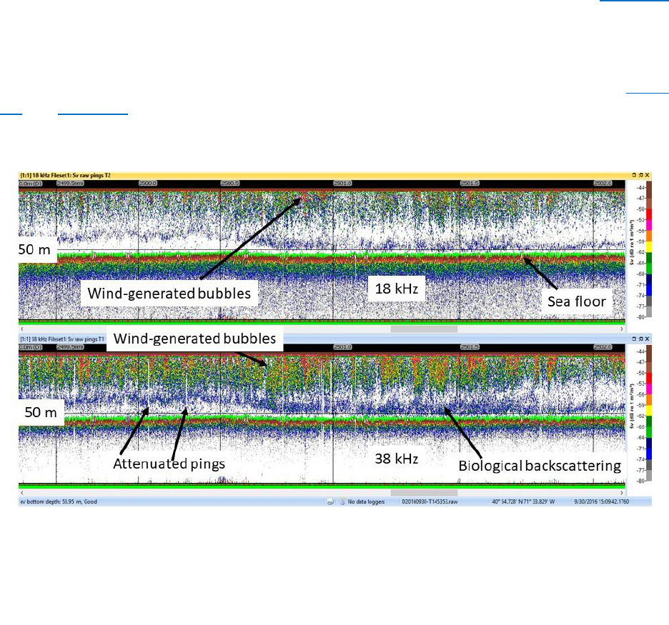
April 2024 84

to encompass near-surface bubbles when they occur due to inclement weather (see Figure 4.5

for an example of near-surface bubbles).

Remove the other main types of noise (impulse, transient, and background) algorithmically from

the data. Generic schemes for removing/minimizing these are given in Peña (2016) and Ryan et

al. (2015). Figure 4.6 and Figure 4.7 provide visual examples of various types of noise, with Figure

4.7 and Figure 4.8 providing detailed examples of the data before and after cleaning using the

techniques described in Ryan et al. (2015).

Figure 4.5. Wind-generated bubble echogram: 18 kHz (upper echogram) and 38 kHz (lower echogram)

data collected on NOAA Ship HB Bigelow during 30 September 2016 showing wind-generated bubbles

extending to about 40 meters depth and attenuated pings (vertical bands of empty scattering in the

38-kHz echogram). Data for this figure were collected using a Simrad ek60. (Image source: NOAA

National Marine Fisheries Service)

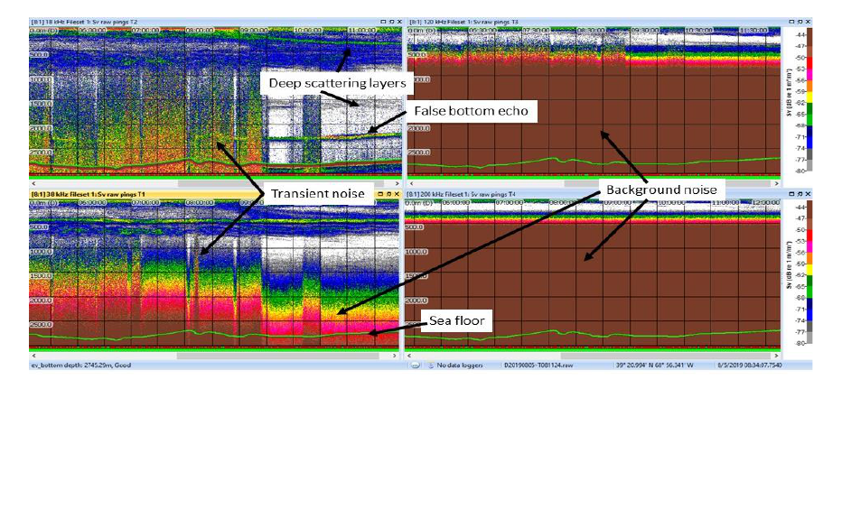
April 2024 85

Figure 4.6. Transient and background noise echogram: 18 kHz (upper left), 38 kHz (lower left), 120 kHz

(upper right), and 200 kHz (lower right) data collected during 5 August 2019 showing transient and

background noise, and a false-bottom echo (aka ghost echo). The portion of the echograms with less

transient noise were collected during a midwater trawl haul. Data for this figure were collected using

a Simrad ek60. (Image source: NOAA National Marine Fisheries Service)

April 2024 86

Figure 4.7. Echograms before and after noise reduction: 18 kHz data collected during 28 July 2019

showing impulse noise from an ultra-short baseline (USBL) acoustic system, a false-bottom echo, and

transient noise due to increased vessel speed (upper echogram), and the same echogram after noise

reduction using algorithms described in Ryan et al. (2015) (lower echogram). The portion of the upper

echogram not infested with transient noise was collected during a NOAA midwater trawl haul. Data

for this figure were collected using a Simrad ek60. (Image source: NOAA National Marine Fisheries

Service)

April 2024 87

Figure 4.8. Removing transient and background noise: 18 kHz (upper left), 38 kHz (lower left), 120 kHz

(upper right), and 200 kHz (lower right) data collected during 5 August 2019 showing results of

applying Ryan et al. (2015) algorithms to remove transient and background noise (compared to Figure

4.6). The 18 kHz echogram shows the remnants of the false-bottom echo, which could be removed

using algorithms developed by Blackwell et al. (2019). Data for this figure were collected using a

Simrad ek60. (Image source: NOAA National Marine Fisheries Service)

April 2024 88

4.6.1 Vessel Speed

Vessel speed can affect data quality, primarily when the transducers are located on the hull and

are susceptible to bubble sweep (i.e., bubbles entrained under the hull and transported across

the transducer faces) or when transducer cables and echosounder electronics are sensitive to

electronic or mechanical noise caused by increased load on engines and generators. Conduct

these tests to measure noise levels at various vessel speeds. For these tests, place the

echosounders into passive mode (no transmit, just reception) and vary the vessel speed (Figure

4.9). The influence of vessel speed can also be observed during active transmissions, especially

in deep water (Figure 4.10). Higher vessel speeds result in higher transient noise. See section

2.5.2.5 for additional information.

Figure 4.9. Speed vs. Noise: results of increasing vessel speed (top graph) on received noise (lower

image) of the multibeam on NOAA Ship Okeanos Explorer. The warmer the colors, the higher the

received noise. SOG = speed over ground; kts = knots. (Image source: Jerram et al., 2020)

April 2024 89

4.6.2 Sonar Synchronization

Operating multiple echosounders or other acoustically transmitting sensors (e.g., ADCPs, Doppler

speed loggers, fathometers, SBPs, acoustic tracking systems) can cause errant signals to be

detected as interference and noise on the water column systems (i.e., cross-talk). These signals

bias backscatter measurements or produce misleading signals during analysis. In all cases,

reporting and understanding the full complement of sensors operating during a mission is key to

providing sufficient context for later data analysis and interpretation.

Many modern echosounders have built-in pulse synchronization options with customized

settings to synchronize and control pulse transmission when multiple transducers are operating

simultaneously. Pulse transmission (or ‘ping timing’) control software can advance or delay

transmitted pulses to minimize or eliminate cross-talk between systems (Figure 4.11). During

hydrographic surveys, the MBES is often the primary sensor, and water column echosounders

are secondary sensors. Synchronization systems provide ping trigger delays to the secondary

echosounders to reduce noise, particularly transmissions from the secondary systems that may

impact the derivation of seafloor depth or backscatter with the primary system (i.e., multibeam).

Figure 4.10. Influence of vessel speed on transient noise: 18 khz data (lower echogram) and

corresponding vessel speed (upper image) collected during 28 July 2019 showing the influence of vessel

speed on transient noise. The vessel speed color scale ranges from 0 kts (red) to 15 kts (blue). Data

were collected using a Simrad ek60. See Figure 4.7 for description of acoustic scattering features.

Higher vessel speeds have greater transient noise. (Image source: NOAA National Marine Fisheries)

Service)

April 2024 90

Water column backscatter data from MBES can be viewed by ping as a “beam fan” (Figure 4.12)

during data acquisition, analysis, and interpretation. The properties of the transmitted pulse in a

hydrographic multibeam system result in some cross-talk across the detected beams. The

seafloor region facing the echosounder (i.e., typically near the nadir or directly beneath the

system) provides a significant return strength (specular reflection). The strength of this return is

apparent on the side lobes of the multiple RX beams, causing a prominent arch of noise at the

same range as the seafloor (known as the nadir ring). The area between the arch (or nadir ring)

and the seafloor is often significant enough to occlude lower strength scatterers like fish (Figure

4.12) and limits the sampling volume for detecting water column features. While methods can

be used to reduce the side lobe effect (Bourguignon et al., 2009), the backscattering strength of

targets below the side lobe effect will be biased. Some multibeam fishery systems use split-

aperture techniques and beamforming to reduce side lobe interference across multiple beams.

Figure 4.11. An image displaying examples of cross-talk between acoustic systems: for this example,

NOAA Ship Okeanos Explorer had two systems (a multibeam and a 70 khz SBES) that were pinging at

the same time. By delaying and synchronizing the ping rates of the two systems the interference

between the systems changed. Data were collected using a Simrad ek80. (Image source: NOAA Office

of Ocean Exploration and Research; Hoy, 2019)

April 2024 91

Noise can also be detected in multibeam data from asynchronous pulses from other acoustic

sources, appearing as rings in the beam fan. These pulses can contribute to errant seafloor

soundings or biased backscatter signals in hydrographic data acquisition.

4.7 Data Formats

The native formats of water column sonar files are proprietary and binary. Such file formats are

not easily handled; however, a recent effort by the fisheries acoustics community resulted in the

creation of netCDF4 files (Macaulay and Peña, 2018) upon the acquisition of an omnidirectional

sonar (Peña et al., 2021). Developing an open-source data format was completed in collaboration

with the academic community and sonar manufacturers. The scientific community continues to

lead the way towards a change in data acquisition format. Through a standard file format, the

data become more accessible to the scientific community and non-experts and better support

FAIR (Findability, Accessibility, Interoperability, and Reusability) data standards (GitHub ices-

eg/wg_WGFAST, 2022). Another benefit of open-source formats is alleviating the burden of

navigating file format changes by the manufacturer. Further, netCDF and cloud-friendly formats,

such as Zarr, facilitate the application of AI and scalable cloud processing, which are becoming

increasingly necessary as data rates increase.

Water column sonar storage rates vary significantly across echosounder systems, operating

frequency, depth or range, and transmitted pulse characteristics. For example, narrowband SBES

surveying in 500 meters water depth using a 1 ms pulse can provide 2 MB/min, whereas a

Figure 4.12. Fish detection in beam fans: example single ping “beam fan” from an MBES showing

detections of the seafloor, a school of fish in the water column, the side lobe seafloor detection, and

likely detection of a fish school within the seafloor detected in the side lobes. (Image source: NOAA

National Centers for Coastal Ocean Science)

April 2024 92

broadband echosounder at the same frequency and pulse length can generate over 86 MB/min.

MBES storage can exceed that of SBES by several orders of magnitude and multibeam data

collection for only seafloor sampling by two orders of magnitude (Rice and Greenway, 2017). A

200-400 kHz MBES sampling less than 50 meters depths can generate data at 30 GB/hour,

whereas a 200 kHz system sampling greater than 100 meters depths will generate about 5

GB/hour (Figure 4.13). The decrease in data rates with depth is not continuous but instead

related to a system’s preconfigured settings that automatically increase the pulse length

stepwise to optimize the signal to noise and resolution of depth detections. A longer pulse length

requires coarser digital sampling of the returning pulse for storage.

4.8 Data Interpretation and Derived Products

Processing raw water column sonar files requires specialized software and/or expert knowledge

of programming and the complexities of the sonar file structure. Software dedicated to

processing these complex files is available commercially and in open-source formats. Echoview

(Echoview Software, 2023) and Large Scale Survey System (MAREC, n.d.) are widely used

commercial software packages with visualization and analytical capabilities. Fledermaus’

Midwater Tool is another option focusing on the visualization of water column data (QPS, 2023).

Open-source code bases have been developed by experts in the community and distributed for

broader use. The deepwater fisheries acoustics team at New Zealand's National Institute of

Water and Atmospheric Research has developed ESP3, a Matlab-based software package

available as source code and compiled for the non-Matlab user (Ladroit et al., 2020). Python-

based software packages called PyEcholab (GitHub CI-CMG/pyEcholab, 2022) and Echopype (Lee

Figure 4.13. MBES frequencies and depths graph: example data rates for an MBES operating at three

frequencies and varying depth ranges (Rice and Greenway, 2017).

April 2024 93

et al., 2020) were developed by scientists at NOAA National Marine Fisheries Alaska Fisheries

Science Center and the University of Washington, respectively. Code bases in R are also available

including EchoR developed by scientists at Institut Français de Recherche pour l'Exploitation de

la Mer (Ifremer) (EchoR, 2022). These are just a few open-source repositories available to read

and process water column sonar data. A more comprehensive list found on the ICES GitHub site

will continue to be updated by the Working Group on Fisheries Acoustics, Science and Technology

with community input (GitHub ices-eg/wg_WGFAST, 2022).

There has been an exponential growth in the volume of water column sonar data collected over

the past decade attributed to collecting data on opportunistic sailings, increased numbers of

sonar-integrated uncrewed vehicles, and new data-intensive sonar systems. Interpretation or

classification of features in the water column has relied on manual assignment or statistical

methods for classification based on geometric form or frequency-dependent backscatter

response (Kloser et al., 2002; Korneliussen et al., 2008; De Robertis et al., 2010; Campanella and

Taylor, 2016). Scientists’ ability to continue relying on manual scrutiny or methods with limited

automation to analyze the new volumes of data collected is quickly diminishing. The

advancement of accessible AI tools in the last few years has opened many new possibilities for

the application of machine learning (ML) and deep learning (DL) models, facilitated by cloud

infrastructure and scalable compute engines, to complex scientific challenges (de La

Beaujardière, 2019; Malde et al., 2020). The challenges faced in efficiently and effectively

processing water column sonar data are well suited to ML/DL methods (Malde et al., 2020;

Michaels et al., 2019).

Although cloud-based processing enables scientists to bring the processing to the data, note that

processing routines designed for a single desktop will likely need to be altered to optimally and

cost-effectively take advantage of a cloud environment. Some recent advances in the application

of ML on water column sonar data include a comparison of different DL models to classify targets

from underwater sonar data (Yue et al., 2017); the use of deep convolutional neural networks for

acoustic target classification (specifically, lesser sand eels of the species Ammodytes marinus;

Brautaset et al., 2020); water column pattern decomposition from stationary sonars using

principal component analysis and nonnegative matrix factorization (Lee and Staneva, 2020); and

the use of supervised learning to facilitate classification, specifically of the seafloor (Sarr et al.,

2021).

4.9 Data Management

The long-term stewardship and centralized access to historical, ongoing, and future water column

sonar datasets are crucial to obtaining the most information and value from these essential data.

The NOAA NCEI has established an archive dedicated to these data where the continually growing

volume and diversity of archived data are globally accessible through the archive’s web-based

map viewer and Amazon Web Services bucket (NCEI, 2021).

For specific details and guidelines on how and where to archive water column sonar data, please

see Section 1.6.3.

April 2024  94 
 
4.10 References 
Anderson, J.T., Van Holliday, D., Kloser, R., Reid, D.G., and Simard, Y. 2008. “Acoustic seabed 
classification: current practice and future directions.” ICES Journal of Marine Science. 
65(6). https://doi.org/10.1093/icesjms/fsn061.  
Benoit-Bird, K.J. and W.W. Au. 2009. “Cooperative prey herding by the pelagic dolphin, Stenella 
longirostris.” The Journal of the Acoustical Society of America. 125(1): 125-137. 
https://doi.org/10.1121/1.2967480. 
Benoit-Bird, K.J. and G.L. Lawson. 2016. “Ecological insights from pelagic habitats acquired using 
active acoustic techniques.” Annual Review of Marine Science. 8: 463-490. 
https://doi.org/10.1146/annurev-marine-122414-034001. 
Blackwell, R., R. Harvey, B. Queste, B. and S. Fielding. 2019. “Aliased seabed detection in 
fisheries acoustic data.” arxiv.org. April 24, 2019. 
https://doi.org/10.48550/arXiv.1904.10736. 
Brandt, S. B. 1996. “Acoustic Assessment of Fish Abundance and Distribution.” In Fisheries 
Techniques (2nd Edition), edited by B.R. Murphy and D.W. Willis. Bethesda: American 
Fisheries Society. 
https://www.scirp.org/reference/referencespapers?referenceid=1759633 
Brautaset, O., A.U. Waldeland, E. Johnsen, K. Malde, L. Eikvil, A.B. Salberg, and N.O. Handegard. 
2020. “Acoustic classification in multifrequency echosounder data using deep 
convolutional neural networks.” ICES Journal of Marine Science, 77(4): 1391-1400. 
https://doi.org/10.1093/icesjms/fsz235. 
Bourguignon, S., L. Berger, C. Scalabrin, R. Fablet, and V. Mazauric. 2009. “Methodological 
developments for improved bottom detection with the ME70 multibeam echosounder.” 
ICES Journal of Marine Science. 66: 1015-1022. https://doi.org/10.1093/icesjms/fsp089. 
Campanella, F. and J. C. Taylor. 2016. “Investigating acoustic diversity of fish aggregations in 
coral reef ecosystems from multifrequency fishery sonar surveys.” Fisheries Research. 181: 
63-76. https://doi.org/10.1016/j.fishres.2016.03.027. 
Colbo, K., Ross, T., Brown, C., and T. Weber. 2014. “A review of oceanographic applications of 
water column data from multibeam echosounders.” Estuarine, Coastal and Shelf Science. 
145: 41-56. https://doi.org/10.1016/j.ecss.2014.04.002. 
Cornell University & New York Sea Grant. n.d. a. “Sampling Effort.” Acoustics Unpacked: A 
General Guide for Deriving Abundance Estimates from Hydroacoustic Data. 
http://www2.dnr.cornell.edu/acoustics/SurveyDesign/Effort.html. 
Cornell University & New York Sea Grant. n.d. b. “Introduction.” Acoustics Unpacked: A General 
Guide for Deriving Abundance Estimates from Hydroacoustic Data. 
www2.dnr.cornell.edu/acoustics/acousticsunpacked.html. 
Cutter, Jr, G.R., and Demer, D.A. 2014. “Seabed classification using surface backscattering 
strength versus acoustic frequency and incidence angle measured with vertical, split-beam 
echosounders.” ICES Journal of Marine Science. 71(4): 882–894. 
https://doi.org/10.1093/icesjms/fst177.  
de La Beaujardière, J. 2019. “A geodata fabric for the 21st century.” Eos, November 25, 2019. 
https://eos.org/features/a-geodata-fabric-for-the-21st-century. 

April 2024  95 
 
Demer, D.A., Berger, L., Bernasconi, M., Bethke, E., Boswell, K., Chu, D., Domokos, R., et al. 
2015. Calibration of Acoustic Instruments. ICES Cooperative Research Report No. 326. 
http://dx.doi.org/10.25607/OBP-185.   
De Robertis, A., and I. Higginbottom. 2007. “A post-processing technique to estimate the signal-
to-noise ratio and remove echosounder background noise.” ICES Journal of Marine 
Science. 64: 1282–1291. https://doi.org/10.1093/icesjms/fsm112. 
De Robertis, A., D.R. McKelvey, and P.H. Ressler. 2010. “Development and application of an 
empirical multifrequency method for backscatter classification.” Canadian Journal of 
Fisheries and Aquatic Sciences. 67(9): 1459-1474. https://doi.org/10.1139/F10-075. 
Echoview Software. 2023. “The world’s premier software package for hydroacoustic data 
processing.” https://www.youtube.com/watch?v=IGo6x_uzG8Y, 
EchoR. 2022. “EchoR”. https://gitlab.ifremer.fr/md0276b/echor. 
FAO. 1983. “Fisheries Acoustics: A Practical Manual for Aquatic Biomass Estimation.” FAO 
Fisheries Technical Paper 240 FIRM/T240. http://www.fao.org/3/x5818e/x5818e00.htm. 
GitHub CI-CMG/pyEcholab. 11 January 2022. “pyEcholab.” https://github.com/CI-
CMG/pyEcholab/  
GitHub ices-eg/wg_WGFAST. 30 June 2022. “Working Group on Fisheries Acoustics, Science and 
Technology.” https://github.com/ices-eg/wg_WGFAST. 
Hoy, S. 2019. “2019 RVTEC Meeting - Breakout10: NOAA SHIP Okeanos Explorer Sonar 
Synchronization.” 
https://www.unols.org/sites/default/files/201910rvt_breakout10_ekfmtradeoffs.pdf.  
ICES. 2015. “SISP 9 - Manual for International Pelagic Surveys (IPS).” Series of ICES Survey 
Protocols (2012–2020). https://doi.org/10.17895/ices.pub.7582 
Jech, J. M., W. Michaels, and C. Wilson. 2007. “Improving Fisheries with Advanced Technology.” 
In Our Living Oceans: Report on the Status of U.S. Living Marine Resources. NOAA 
Technical Memorandum NMFS-F/SPO-80. 
https://spo.nmfs.noaa.gov/sites/default/files/tm80.pdf. 
Jech, J. M., Schaber, M., Cox, M., Escobar-Flores, P., Gastauer, S., Haris, K., Horne, J., et al. 2021. 
“Collecting quality echosounder data in inclement weather.” ICES Cooperative Research 
Report. 352: 108. https://doi.org/10.17895/ices.pub.7539.  
Jerram, K., S. Hoy, and C. Wilkins. 2020. “Okeanos Explorer EX2000 EM304 Sea Acceptance 
Testing.” 
https://mac.unols.org/sites/mac.unols.org/files/EX2000_EM304_SAT_FINAL_v3_2020032
5_Redacted.pdf.  
Joye, S. B. 2015. “Deepwater Horizon, 5 Years On.” Science. 349: 592–593. 
https://doi.org/10.1126/science.aab4133. 
Kloser, R.J., Ryan, T., Sakov, P., Williams, A., and Koslow, J.A.. 2002. “Species identification in 
deep water using multiple acoustic frequencies.” Canadian Journal of Fisheries and 
Aquatic Sciences. 59(6): 1065-1077. https://doi.org/10.1139/f02-076. 
Korneliussen, R.L., N. Diner, E. Ona, L. Berger, and P.G. Fernandes. 2008. “Proposals for the 
Collection of Multifrequency Acoustic Data.” ICES Journal of Marine Science. 65(6): 982–
994. https://doi.org/10.1093/icesjms/fsn052. 

April 2024  96 
 
Koslow, J. A., 2009. “The role of Acoustics in Ecosystem-Based Fishery Management.” ICES 
Journal of Marine Science. 66(6): 966–973. https://doi.org/10.1093/icesjms/fsp082.  
Ladroit, Y., P.C. Escobar-Flores, A.C. Schimel, and R.L. O’Driscoll. 2020. “ESP3: An Open-Source 
Software for the Quantitative Processing of Hydro-Acoustic Data.” SoftwareX. 12: 100581. 
https://doi.org/10.1016/j.softx.2020.100581. 
Ladroit, Y., G. Lamarche, and A. Pallentin. 2018. “Seafloor Multibeam Backscatter Calibration 
Experiment: Comparing 45°-tilted 38-kHz Split-Beam Echosounder and 30-kHz Multibeam 
Data.” Marine Geophysical Research. 39: 41–53. https://doi.org/10.1007/s11001-017-
9340-5. 
Lanzoni, C. and T. C. Weber. 2011. “A Method for Field Calibration of a Multibeam 
Echosounder.” OCEANS'11 MTS/IEEE KONA, Waikoloa, HI, USA. 
https://doi.org/10.23919/OCEANS.2011.6107075. 
Lee, W. J. and V. Staneva. 2020. “Compact representation of temporal processes in 
echosounder time series via matrix decomposition.” The Journal of the Acoustical Society 
of America. 148(6): 3429-3442. https://doi.org/10.1121/10.0002670. 
Lee, W. J., K. Nguyen, and V. Staneva. 2020. “Echopype: Enabling interoperability and scalability 
in ocean sonar data analysis (v0.4.0).” https://zenodo.org/record/3907000#.Y8_lg3bMKUl. 
Lurton, X. 2002. An Introduction to Underwater Acoustics: Principles and Applications. 
Heidelberg, Springer Berlin. https://link.springer.com/book/9783540784807. 
Macaulay, G. and H. Peña. 2018. “The SONAR-netCDF4 convention for sonar data, Version 1.0.” 
ICES Cooperative Research Report. https://doi.org/10.17895/ices.pub.4392. 
Malde, K., N.O. Handegard, L. Eikvil, and A.B. Salberg. 2020. “Machine intelligence and the data-
driven future of marine science.” ICES Journal of Marine Science. 77(4): 1274-1285. 
https://doi.org/10.1093/icesjms/fsz057. 
MAREC. n.d. “Home.” https://www.marec.no. 
McConnaughey, R.A. and Syrjala, S.E. 2009. “Statistical relationships between the distributions 
of groundfish and crabs in the eastern Bering Sea and processed returns from a single-
beam echosounder.” ICES Journal of Marine Science. 66(6): 1425-1432. 
https://doi.org/10.1093/icesjms/fsp147. 
Michaels, W.L., Handegard, N.O., Malde, K. & Hammersland-White, H. 2019. Machine Learning 
to Improve Marine Science for the Sustainability of Living Ocean Resources: Report from 
the 2019 Norway - U.S. Workshop. NOAA Tech. Memo. NMFS-F/SPO-199. 
https://spo.nmfs.noaa.gov/sites/default/files/TMSPO199_0_0.pdf.  
National Ocean Mapping, Exploration, and Characterization Council of the Ocean Science and 
Technology Subcommittee and Ocean Policy (NOMEC). 2020. Implementation Plan for the 
National Strategy for Ocean Mapping, Exploring, and Characterizing the United States 
Exclusive Economic Zone Committee. https://trumpwhitehouse.archives.gov/wp-
content/uploads/2020/01/210107-FINAL-NOMEC-Implementation-Plan-Clean.pdf. 
NOAA NCEI. 25 March 2021. “Understanding Our Ocean with Water-Column Sonar Data.” 
https://storymaps.arcgis.com/stories/e245977def474bdba60952f30576908f?fbclid=IwAR
1mEflE1Nk5285GRiqMtYC70Q-4z4xNT8H6HuKhUnsbMgqelXPpht8Nu2I. 
NOAA OER. 2020. NOAA OER Deepwater Exploration Mapping Procedures Manual. 
https://doi.org/10.25923/jw71-ga98.   

April 2024  97 
 
Parker-Stetter, S.L., Rudstam, L.G., Sullivan, P.J., and Warner, D.M. 2009. Standard Operating 
Procedures for Fisheries Acoustic Surveys in the Great Lakes. Great Lakes Fish. Comm. 
Spec. Pub. 09-01. http://www.glfc.org/pubs/SpecialPubs/Sp09_1.pdf. 
Peña, H., Macaulay, G. J., Ona, E., Vatnehol, S., and Holmin, A. J. 2021. “Estimating individual 
fish school biomass using digital omnidirectional sonars, applied to mackerel and herring.” 
ICES Journal of Marine Science. 78(3): 940-957. https://doi.org/10.1093/icesjms/fsaa237. 
Peña, M. 2016. “Incrementing data quality of multi-frequency echograms using the Adaptive 
Wiener Filter (AWF) denoising algorithm.” Deep-Sea Research I. 116: 14-21. 
https://doi.org/10.1016/j.dsr.2016.07.008.  
Proni, J. R., and J R. Apel. 1975. “On the Use of High-Frequency Acoustics for the Study of 
Internal Waves and Microstructure.” Journal of Geophysical Research.  80(9): 1147-1151. 
https://doi.org/10.1029/JC080i009p01147.  
Quality Positioning Services (QPS). 2023. “Fledermaus: 4D geo-spatial analysis.” 
https://www.qps.nl/fledermaus. 
Ryan, T. E., Downie, R. A., Kloser, R. J., Keith, G. 2015. “Reducing bias due to noise and 
attenuation in open-ocean echo integration data.” ICES Journal of Marine Science. 72(8): 
2482-2493. https://doi.org/10.1093/icesjms/fsv121.  
Rice, G. and Greenaway, S. 2017. “NOAA SHIP FAIRWEATHER Launch 2805, 2806, 2807, AND 
2808 EM2040 Acceptance Testing.” 
https://mac.unols.org/sites/mac.unols.org/files/Fairweather_Launch_EM2040_Acceptanc
e.pdf. 
Sarr, J.M.A., Brochier, T., Brehmer, P., Perrot, Y., Bah, A., Sarré, A., Jeyid, M.A., Sidibeh, M. and 
El Ayoubi, S., 2021. “Complex data labeling with deep learning methods: Lessons from 
fisheries acoustics.” ISA transactions. 109: 113-125. 
https://doi.org/10.1016/j.isatra.2020.09.018. 
Skarke, A., Ruppel, C., Kodis, M. et al. 2014. “Widespread methane leakage from the seafloor on 
the northern US Atlantic margin.” Nature Geoscience. 7: 657–66. 
https://doi.org/10.1038/ngeo2232. 
Stienessen, S., N. Lauffenburger, and A. De Robertis. 2019. “Results of the acoustic-trawl 
surveys of walleye pollock (Gadus chalcogrammus) in the Gulf of Alaska, February-March 
2018 (DY2018-01 and DY2018-03).” NOAA, National Marine Fisheries Service. 
https://doi.org/10.25923/rt3f-b427. 
Stranne, C., Mayer, L., Weber, T.C., Ruddick, B.R., Jakobsson, M., Jerram, K., Weidner, E., 
Nilsson, J. and Gårdfeldt, K. 2017. “Acoustic mapping of thermohaline staircases in the 
Arctic Ocean.” Scientific Reports, 7(1): 1-9. https://doi.org/10.1038/s41598-017-15486-3. 
Stranne, C., Mayer, L., Jakobsson, M., Weidner, E., Jerram, K., Weber, T.C., Anderson, L.G., 
Nilsson, J., Björk, G. and Gårdfeldt, K., 2018. “Acoustic mapping of mixed layer depth.” 
Ocean Science. 14(3): 503-514. https://doi.org/10.5194/os-14-503-2018. 
Tournier, Martin, Goulet, Pauline, Fonvieille, Nadège, Nerini, David, Johnson, Mark, and 
Christophe Guinet. 2021. “A novel animal-borne miniature echosounder to observe the 
distribution and migration patterns of intermediate trophic levels in the Southern Ocean.”  
Journal of Marine Systems. https://doi.org/10.1016/j.jmarsys.2021.103608. 

April 2024  98 
 
Trenkel, V. M., Mazauric, V. and L. Berger. 2008. “The new fisheries multibeam echosounder 
ME70: description and expected contribution to fisheries research.” ICES Journal of Marine 
Science. 65:645-655. https://doi.org/10.1093/icesjms/fsn051. 
Watkins, J. and J.L. Worzel. 1978. “The serendipity gas seep area, south Texas offshore.” 
American Association of Petroleum Geologists Bulletin. 62: 1067-1074. 
https://doi.org/10.1306/C1EA4F95-16C9-11D7-8645000102C1865D. 
Webb, T. J., Berghe, E. V., & Odor, R. 2010. “Biodiversity’s Big Wet Secret: The Global 
Distribution of Marine Biological Records Reveals Chronic Under-Exploration of the Deep 
Pelagic Ocean.” PLoS ONE. 5(8). https://doi.org/10.1371/journal.pone.0010223.  
Weber, T. C., Jerram K., & Mayer L. 2012. “Acoustic sensing of gas seeps in the deep ocean with 
split-beam echosounders.” Proceedings of Meetings on Acoustics. 17, 070057. 
https://doi.org/10.1121/1.4772948.  
Yue, H., Zhang, L., Wang, D., Wang, Y. and Lu, Z., 2017. “The classification of underwater 
acoustic targets based on deep learning methods.” 2nd International Conference on 
Control, Automation and Artificial Intelligence. Atlantis Press. 
https://dx.doi.org/10.2991/caai-17.2017.118. 
 
   

April 2024 99

Chapter 5: Side Scan Sonar

Chris Gardner, NOAA

Martha Herzog, NOAA

Steven Intelmann, NOAA

Monique LaFrance Bartley, NPS

James J. Miller, NOAA

Jennifer Miller, BOEM

Paul Turner, NOAA

Matthew Wilson, NOAA

5.1 Introduction

SSS are acoustic instruments that transmit two narrow, fan-shaped beams in a wide track on both

sides of a path (Figure 5.1). The beams radiate from the sonar’s transducers to the seafloor; the

transducers also record the returns as a series of backscatter vs. time measurements. The sound

is absorbed, reflected, and scattered to various degrees, depending on the seafloor’s geological,

geomorphic, and biological characteristics and anthropogenic features (e.g., shipwrecks,

obstructions). For example, soft sediment environments absorb more sound than coarse

sediment and rocky environments, coral reefs and shellfish beds, and shipwrecks, all of which

tend to reflect sound. The unique acoustic pattern indicative of a given seafloor feature is

referred to as its “acoustic signature” and allows for the side scan data to be interpreted. The

relief of seafloor features is calculated by measuring the shadow height in the side scan record.

SSS can be towed at depth behind a vessel or operated from AUVs at a fixed altitude above the

seafloor (Figure 5.2). Hull mounted SSS are also used, generally in shallower water.

SSS data have broad applicability, and surveys are conducted to meet project goals that range

from seafloor characterization (e.g., benthic habitats, sediment, geologic and geomorphic

features) to supplementing hydrographic surveys to meet object detection requirements (e.g.,

used in the region between regular MBES sounding lines for the additional indication of dangers

and bathymetric irregularities).

This chapter focuses on collecting, processing, and delivering SSS data and will summarize best

practices for acquisition standards and system set-up, range scales, frequencies and ping rates,

coverage requirements, positioning, system calibration, QA/QC techniques, and how to derive

products. This chapter provides overarching guidance and recommendations and will not address

manufacturer-specific recommendations or recommendations concerning specific use cases.

5.1.1 Data Management

Management of SSS data is necessary for efficient use, future access, and validation of analytical

and interpretative results. Record SSS raw data files in the instrument’s vendor-specific format.

Common file formats include, but are not limited to .xtf, .jsf., .hsx, and .gcf. Archive the raw and

processed data (i.e., mosaics) to ensure data are preserved to the fullest extent.

For specific details and guidelines associated with minimum SSS data requirements and

management (recommended file formats, metadata, data archival, etc.), see Chapter 1.6.4.

April 2024 100

5.1.2 Raw Data Acquisition

Below is essential information to be confirmed in data files and/or survey reports to increase

usability:

• Sonar settings

o Operational frequency (report both frequencies if using a dual frequency

system)

• Attitude and positioning

o Specifications of the navigation system(s)

o Accuracy

o Installation information

▪ Linear and angular offsets for installation on surface vessels or

underwater vehicles

▪ Towfish configuration and winch/cable information, if towed

Figure 5.1. Schematic of a towed system: towed system and sonar beams (top) and data visualization

(bottom) in which lines of data are interpreted as a “waterfall” image. Image courtesy of USGS.

April 2024 101

• Spatial reference

▪ Coordinate system and horizontal datum references for raw

echosounder data and navigation system, if different

o Options as stated in Lurton and Lamarche (2015):

▪ No geo‐reference

▪ Geographic reference (lat, long)

▪ Projected reference (Mercator, UTM, other projected reference)

▪ Other

5.1.3 Data Processing and Mosaic Generation

Below is essential information to be confirmed in data files and/or survey reports to increase

usability:

• Processing steps

o Describe data processing steps

o Note application of gains (e.g., TVG, angular varying gain [AVG]), lookup tables

(LUT), etc. to correct for water column returns, arrival angle, and refine

contrast to produce a color-balanced image

o Documentation of targets identified, if processed and available

• Spatial reference

o Coordinate system and horizontal datum

o Describe processing used to shift coordinate system or datum, if different from

raw data

o Options as stated in Lurton and Lamarche (2015):

▪ No geo‐reference

▪ Geographic reference (lat, long)

▪ Projected reference (Mercator, UTM, other projected reference)

▪ Other

• Mosaicking settings

o Order (top, bottom)

o Statistical (average)

• Visual representation

o Examples: Greyscale 0‐255, gold scale 0-255, inverse gold scale 0-255

April 2024 102

5.2 Target Detection

The specific settings used to acquire and process side scan data differ depending on project goals

and the equipment and software used. It is recognized that defining a set of standard best

protocols for the mapping community to follow is challenging. Instead, this chapter directs SSS

operators and data processors to operate in such a manner that the data can detect a target (i.e.,

object or feature) of a particular dimension on the seafloor. In water depths less than or equal to

20 m, a target that measures 1 m x 1 m x 1 m (with the height measured from shadow length)

should be detectable. In water depths greater than 20 m, a target should be detectable with a

height (measured from shadow length) of at least 5% of the depth. The settings, software, and

equipment needed to achieve these target detection standards are for the user to determine.

When a target is correlated to multibeam data acquired concurrently with SSS operations,

determine the shallowest depth of the target from the multibeam data. Determine the

shallowest depth measurement from a beam within 30 degrees of nadir unless multiple passes

were made over the target. If the correlating sounding is sourced from one of the outer beams

of the multibeam system, investigate the target further.

Figure 5.2. Side scan sonar examples: side scan towfish, typical towed deployment, raw

sonar backscatter, and photograph of limestone reef at location of side scan imagery.

Images courtesy of NOAA Fisheries.

April 2024 103

5.3 Coverage Requirements

SSS data coverage needs and range scale will vary based on specific program, project goals, and

equipment used. Coverage refers to the extent to which SSS swaths ensonify the seafloor with a

received detection—i.e., the band of the sea bottom that is ensonified and recorded along a

single vessel track line to the detection (e.g., -3 dB) limits. Range scale is the width of the seafloor

ensonified on each side of the SSS towfish along a single vessel track line. The recommended

percent of ensonified seafloor coverage is 125% or greater with 10% or greater overlap between

each vessel trackline. This recommendation balances the desire for the seafloor to be fully

ensonified (i.e., 100% coverage) and survey efficiency/wise expenditure of resources (i.e.,

minimal survey effort to achieve project goals). Note: If the project purpose is for navigation or

object detection, then 125% coverage may not be adequate; refer to the NOAA Hydrographic

Survey Specifications and Deliverables for additional guidance (NOAA OCS, n.d.).

5.4 Spatial Referencing

Survey coverage data should be provided as a geospatial dataset (e.g., .shp, .gdb) that includes

the polygon feature class(es) of the location of the study site(s) surveyed and the line feature

class(es) of the navigational cruise track lines of the survey vessel. If there is more than one study

site, provide cruise track lines as a separate feature class per study site. Merge track line files to

Figure 5.3. Side scan data collection: collection results over artificial reefs (military tanks). Image

courtesy of Florida Fish and Wildlife Research Institute.

April 2024 104

produce a single feature class if multiple line files were recorded for a given study site (e.g., based

on the survey date, a subsection of the larger study site, or individual track lines).

Geospatial data should be georeferenced to the most current horizontal datum from the National

Spatial Reference System. Projection information must be defined in the feature class so that the

data project accurately when imported into GIS.

Geographic data must use the most recent adjustment and epoch of the North American Datum

(NAD) of 1983 (currently NAD83(2011), Epoch 2010.00) in either UTM (eastings/northings) with

the zone specified or as geographic coordinates (latitude/longitude) and adequately

documented. Note: Both horizontal and vertical datums will be replaced by the North American

Terrestrial Reference Frame of 2022 (NATRF2022), based on GPS/GNSS and a GRAV-D-based

geoid (GEOID2022) (NOAA NGS, n.d.).

5.5 General Side Scan Data Acquisition Parameters

The following are standard acquisition parameters to use as a reference for guidance. Use specific

settings to meet the target detection criteria defined above.

5.5.1 Frequency

Signal frequency varies across sonar systems, typically between 100 and 500 kHz for systems

intended for object detection and seafloor characterization. There is a trade-off between lower

and higher frequency systems: lower frequencies offer increased maximum range scale (or swath

width), whereas higher frequencies offer increased image fidelity and resolution.

5.5.2 Navigation/Positional Uncertainty/Accuracy

At a minimum, utilize a position and attitude system with one or more GNSS receivers and an

IMU during a survey. A GNSS receiver acquires the vessel’s position using GNSS satellites (i.e.,

GPS), and when using multiple receivers, it also provides heading information. Use the exact

GNSS clock signal for positioning as the timing signal for the entire survey system. The IMU

measures vessel attitude (i.e., roll, pitch, yaw, and heave) across all axes and rotations. These

data, in conjunction with the positioning data and sound speed, allow data to be corrected to its

true position on the seafloor. In integrated systems, the data from the IMU allows the vessel to

maintain an accurate position, even in the event of a total loss of GNSS satellites for short

durations such as operating under a bridge or other obstructions.

Horizontal accuracy will depend on the system configuration, investigation technique, water

depth, and target density. However, the position of targets identified with side scan imagery must

be sufficiently accurate to relocate the feature.

April 2024 105

5.5.3 Survey Speed

Data collection speed should be such that an object 1 m x 1 m x 1 m would be independently

ensonified a minimum of three times per pass. Typical survey speeds are 3-6 knots, though it

could be faster, as survey equipment and conditions permit.

5.5.4 Horizontal Range

The achievable horizontal range of a SSS is a function of several parameters, including the sonar

system’s characteristics and tow/mount configuration, range scale in use, seafloor composition,

and environmental factors (e.g., sea state, inclement weather, water column). If the effective

range scale of the SSS is reduced due to external factors, then the range scale should be reduced

accordingly to meet the target detection criteria and data coverage needs. For example,

environmental changes may distort the outer half of the 100 m range scale. In this case, only 50

m of effective range could be claimed.

5.6 System Configuration

5.6.1 Towed System

A towed sonar system configuration can significantly reduce the effects of vessel motion and

allow for adjustment of the operating height of the towfish (Figure 5.2) above the seafloor to

enable the optimum shadow, both of which improve data quality and resolution. However, the

disadvantage of towed configurations is that they introduce uncertainty regarding the position

of the towfish. This error has three components:

● An along-track component caused by uncertainty in how far the towfish is astern of the

vessel. This error depends on the length of cable out, depth of towfish, and vertical

catenary of the cable (the last two also vary with the ship’s speed);

● An across-track component, caused by deflection of the towfish by the tidal stream or

current and by ship maneuvers;

● Errors in the position of the ship or boat transferred to the towfish.

For towed sonar systems, measure static vessel offsets to the tow point. Calculate the actual

towfish position using towfish depth and cable-out measurements. Determine towfish depth by

a depth sensor installed in the towfish or calculated by subtracting the towfish height

(determined by a separate echosounder installed in the towfish or the first return of each sonar

ping) from the depth of water (determined from a vessel echosounder). If the sonar is equipped

with a pressure sensor, test its accuracy annually and whenever the horizontal positioning

accuracy of side scan targets is in doubt.

Cable out can be estimated visually from calibrated markings on the cable or measured with an

electronic cable counter. Note: When measuring cable out, the cable zero mark is not at its

connection to the towfish but the phase center of the sonar.

April 2024 106

For most SSS operations, the optimum height of the towfish above the seafloor is 8% to 20% of

the range scale in use. For any towfish height below 8% of the range scale in use, the effective

scanning range is defined to equal 12.5 times the towfish height, provided adequate echoes have

been received. During shallow water operations, the towfish may need to be flown very close to

the surface with little tow-cable out which may introduce noise in the data from surface waves,

and ship wake, and additional survey lines may need to be run to ensure coverage requirements

are met. When the towfish height has exceeded 20% of the range scale, carefully examine the

data, as targets will display reduced shadow length to height.

In sufficiently shallow survey areas (perhaps <500 m), a USBL system can be used to more

accurately position the towfish. Properly installed, calibrated, and processed USBL data can

provide more accurate positioning than a simple cable-out determination of layback. In practice,

USBL systems calculate the subsurface position of an object by combining acoustic range and

bearing data from a vessel-mounted transceiver with attitude, heading, and location information

from the vessel’s navigation system. The tracked object is equipped with an acoustic transponder

or responder that communicates with the transceiver attached to the vessel. This technology

does not require a transponder array to be deployed on the seafloor before positioning can

commence and is thus ideal for trackline surveys. The transceiver can be affixed to the vessel’s

hull or on a stable over-the-side pole with no inherent wobble at survey speed. Hull-mounted

configurations require the transceiver to sit well below the vessel to avoid interference and

multipath conditions. In nearly all cases, the calculated XYZ acoustic positions will require some

degree of post-process smoothing before reinsertion into the raw sonar navigation packets

before mosaicking.

5.6.2 Vessel-Mounted System

Hull-mounted or pole-mounted (bow or side) sonar system configurations allow for the position

and orientation of the sonar to be accurately known, improving the positioning of detected

features in the SSS data. Mounted systems are preferred in shallow waters or areas with potential

or known hazards that pose challenges to surveying with a towed system. For example, mounted

systems reduce the risk of entanglement in fishing gear and making contact with obstructions

(e.g., boulders, wrecks). Mounted systems also increase the freedom of maneuverability of the

survey vessel. Pole-mounted systems provide the benefit of adjustable and repeatable survey

operations, and the systems are quick to set up. Pole-mounted systems are beneficial for mobile

or ‘fly-away’ system configurations.

Position data for hull or pole-mounted SSS systems are typically more accurate than a towed SSS

system configuration, and operations in shallow waters can be conducted with less risk and

increased safety and efficiency compared to towed systems. Range scale requirements for this

configuration are based on a factor of water depth with the towfish height above the bottom to

be 8%–20% towfish height of the operating range scale.

However, mounted configurations may introduce additional vessel motion effects on the data

and potential interference from other vessel-mounted sensors. This method also may limit the

April 2024 107

operational extent of a given sonar system since it is attached to the vessel and unable to be

operated at the optimum height above the seafloor.

For hull-mounted systems, position the sonar’s phase center of the SSS during the vessel static

offsets survey. The phase center of the sonar is considered to be at the fore and aft midpoint of

the transducer and on the centerline in the athwart ship and vertical axes.

For pole-mounted systems, measure and confirm offsets annually. Use the benchmark closest to

the pole mount as a reference point. The X, Y, and Z should be measured from the vessel’s

reference point. Some pole-mounted systems do not require traditional offset measurements

because of their “plug and play” ability. In these setups, the antennas, IMU, and sonar are all

integrated into the single boat setup, making the measurements of the vessel negligible.

5.6.3 Documenting System Configuration

Measure and/or verify SSS system offsets before calibration. Depending upon whether the sonar

configuration is hull-mounted or towed, requirements for offset measurements will vary.

At a minimum, vessel configuration and offset information should be presented as a text file (e.g.,

ASCII) or spreadsheet (e.g., .csv, .xlsx) AND a schematic file (e.g., .jpg, .bmp., .tiff). The files should

contain details of survey vessel dimensions (length, width, draft) and offsets of survey

instruments. Provide multiple files if using more than one vessel or configuration.

5.7 System Calibration

The SSS calibration test should consist of multiple passes (e.g., 10) on a known target. Image the

target from various ranges and directions with survey speed, water depth, and weather

representative of typical survey conditions. When possible and/or necessary to meet project

goals, use an alternate system (e.g., MBES) to determine a high-accuracy absolute position of the

target for comparison with SSS detected positions. Conduct this test across all range scales

intended to be used for data acquisition.

Successful object detections should be used to compare the mean detected position with the

absolute target position and to compute the approximate 95% confidence radius for the system.

This radius should not exceed 5 meters for hull-mounted systems and 10 meters for towed

systems.

Line plans are recommended for conducting a SSS calibration test (Figure 5.4). The recommended

plan balances ensonifications on the port and starboard channels, across the range scale, from

different target aspects, and from different directions, assisting the hydrographer in

differentiating systematic and random errors in detection and positioning.

April 2024 108

5.8 Quality Control

5.8.1 Quality Assurance and Confidence Checks

Conduct confidence checks of the SSS system prior to a survey and at least once daily during a

survey. Accompany these checks at the outer limits of the range scales being used based on a

target near or on the bottom. Check each sonar channel (i.e., port and starboard channels) to

verify proper system tuning and operation. Confidence checks can be made on any discrete

object, offshore structure, or bottom feature convenient or incidental to the survey area. Targets

can include wrecks, offshore structures, navigation buoy moorings, distinct trawl scours, or sand

ripples. If a convenient or incidental target is unavailable, place a known target on or near the

bottom and use it for confidence checks.

Make confidence checks during survey operations by noting the check target on the sonogram.

Confidence checks are an integral part of the daily SSS operation and should be annotated,

including the time of check, in the SSS acquisition and processing logs.

When an area is ensonified multiple times, examine and correlate targets between successive

SSS coverages (i.e., compare the first 100% with the second 100% sonar coverage) or MBES data.

Figure 5.4. Side scan sonar calibration line plan: recommended line plan for SSS calibration testing.

Image courtesy of NOAA Office of Coast Survey.

April 2024 109

Anomalous targets which appear consistently and correlate in each data record provide

increased confidence that the acquisition system(s) is(are) working correctly and help to confirm

the existence of these targets.

Before surveying with an SSS system that has been reconfigured or stored, perform a rub test.

The test consists of manually rubbing each transducer on the towfish while the system is pinging

and confirming the observed side scan return signal in the incoming data stream. A rub test

failure indicates system errors such as incorrect gain or power settings, a faulty cable, or damaged

transducers. Conduct this test swiftly while the towfish is out of the water and dry to avoid the

possibility of electric shock. While testing, avoid running the system for an extended period while

out of the water.

5.8.2 Environmental Influences

Environmental influences can impact the SSS record, including density differences between

water masses, water mass separation and mixing due to tidal flows, surface mirroring (Lloyd

Mirror Effect), and water column interference due to entrained air bubbles (e.g., from passing

vessel prop wash or wave action), suspended sediment, and fish and other biologic organisms.

These influences interfere with seafloor detection and affect the return signal, causing refraction

and distortion in outer swath regions and degrading data quality.

In areas that experience a strong thermocline, sonar operators will need to lower the towfish

below the thermocline so the SSS signal does not pass through the dense thermocline layer. Sea

state can also influence data collection and quality, especially for hull-mounted and pole-

mounted systems operating in surface waters where air bubbles become entrained from wave

action.

SSS records that include environmental influences affecting any portion of the swath and hinder

the selection of contacts in the affected regions do not meet the requirement of 100% complete

coverage. In such cases, reduce the swath range and reject the affected areas. Data should be

reacquired to meet the complete coverage requirement.

5.8.3 Operational Considerations

It is good practice to tow the sonar parallel to the contours in areas characterized by relatively

low gradients. However, when surveying in terrain with steep walls or submarine canyons, higher

quality data are achieved by “flying” the towfish in a downslope direction to avoid the effect of

achieving no acoustic return from the deep-side channel where the signal propagation may not

reach the seafloor to elicit a return echo.

April 2024 110

5.9 Data Products

5.9.1 Mosaics

SSS data are compiled into mosaics of georeferenced sonar imagery (Figure 5.5). These products

are often incorporated into GIS for analysis and visualization. Follow these mosaic protocols to

enable the greatest use of the data:

• A single georeferenced raster file for each area of coverage in floating point GeoTIFF

format or other standard image file format (e.g., JPEG2000).

• The projection information must be defined in the image (e.g., .GeoTIFF) or in an

associated file (e.g., .tif with accompanying .twf file) so that the data project

accurately when imported into GIS.

• SSS data should be presented as a continuous and comprehensive “map view” by

“stitching” together adjacent individual track lines of processed data.

• Merge overlapping data to produce the best visual display; options include averaging

and ordering by timestamp.

• Visual data products should use a color scheme standard in the industry (e.g.,

grayscale, inverse grayscale, gold scale).

• Tile mosaics, if necessary (e.g., for large study sites), to reduce file size and improve

the visual layout of maps.

• SSS mosaics and waterfall images should represent data that have been processed to

remove the central nadir region and at a color scale that enhances feature

identification.

April 2024 111

5.10 Other Resources

SOPs have been developed for SSS operations, and some example protocols and websites with

further guidance are listed below:

• NOAA Hydrographic Survey Specifications and Deliverables (NOAA OCS, n.d.)

• NOAA Field Procedures Manual (NOAA OCS, n.d.)

• IHO S-44 Chapter 4 Seafloor Classification (IHO, n.d.)

• Procedures and Criteria for Evaluating Benthic Mapping Data (LaFrance et al., 2019)

Figure 5.5. Geotiff mosaic of side scan sonar data collected with an AUV mounted system: imagery

depicts several low-relief rocky reefs, a limestone ledge, and adjacent sand habitats. Image courtesy

of NOAA Fisheries.

April 2024 112

5.11 References

IHO. n.d. “Chapter 4: Seafloor Classification and Feature Detection.”

https://iho.int/uploads/user/pubs/cb/c-13/english/C-13_Chapter_4.pdf.

LaFrance Bartley, M., T. Curdts, and S. Stevens. 2019. Procedures and Criteria for Evaluating

Benthic Mapping Data: A Northeast Coastal and Barrier Network Methods Document.

Natural Resource Report NPS/NCBN/NRR—2019/2050. National Park Service, Fort Collins,

Colorado. https://irma.nps.gov/DataStore/DownloadFile/633175.

Lurton, X. and G. Lamarche. 2015. Backscatter Measurements by Seafloor‐Mapping Sonars:

Guidelines and Recommendations. https://geohab.org/wp-

content/uploads/2018/09/BWSG-REPORT-MAY2015.pdf.

NOAA NGS. n.d. “New Datums.” National Geodetic Survey.

https://www.ngs.noaa.gov/datums/newdatums/index.shtml

NOAA OCS. n.d. “Standards and Requirements.”

https://nauticalcharts.noaa.gov/publications/standards-and-requirements.html.

April 2024 113

Chapter 6: Sub-bottom Profiling

Jeff Danielson, USGS

Chris DuFore, BOEM

Jim Flocks, USGS

Arnell Forde, USGS

Dave Foster, USGS

Jenna Hill, USGS

Jennifer Miller, BOEM

Jeff Waldner, BOEM

6.1 Introduction

Sub-bottom (subseafloor) profiles are acquired using seismic-reflection techniques that provide

a continuous vertical two-dimensional (2D) stratigraphic display along the survey ship’s track.

Interpretation and analysis of these profiles are used to map shallow (generally less than 200 m)

stratigraphic and morphologic features. Sub-bottom systems use an acoustic source to transmit

a sound wave directed downward. These systems work the same as bathymetric sensors but are

of lower frequency so that the signal penetrates the seafloor, where it responds to density or

sound speed changes in the sub-bottom structure through an acoustic impedance. The acoustic

impedance (z) of a material is defined by the product of sound speed and density of the material.

Some of the transmitted acoustic waves reflect where there is a contrast acoustic impedance

(e.g., the contact between the water column and seafloor). Some of the transmitted waves

propagate through the seafloor and sediment. The depth of penetration of the acoustic energy

below the seafloor and the sub-bottom depends on the power and frequency of the acoustic

source and the acoustic impedance of the substrate. Seafloor and sub-bottom reflections are

received either by the acoustic source (transducer) or a separate receiver (hydrophone) and

recorded digitally as amplitude and source to receiver time (two-way travel time). Reflectivity

and timing of the return signal are processed through topside hardware to produce a vertical, 2D

profile of the subsurface physical environment as a series of amplitude changes over time and

distance. Numerous publications describe 2D seismic data acquisition in the marine environment

in detail (e.g., Dondurur, 2018).

This chapter describes SOPs for using one receiver (single-channel seismic [SCS]) within frequency

bandwidths ranging from 0.2 kHz to 24 kHz. Sub-bottom systems can have a separate source and

receiver, or the source can also act as a receiver (transducer). The term sub-bottom often refers

to systems where the source and receiver are a single component, or the source and receiver are

both contained within a tow vehicle. In this chapter, we also use the term sub-bottom to describe

systems with sources and receivers that are towed separately. These acoustic sources are often

referred to as high-resolution geophysical (HRG) sources, typically used in shallow subseafloor

imaging and have lower power and higher frequencies than implosive type systems (airguns).

Airguns are more typically used with multichannel seismic (MCS) systems, which have multiple

receivers offset by distance from acoustic sources. MCS systems are not addressed in this chapter

due to the complexity of acquisition, processing, and survey-specific design. However, much of

the SOP for SCS applies to MCS systems. Boomer and sparker sound sources are increasingly

paired with multichannel streamers for very high-resolution continental shelf surveys, for

example, 32 channels (groups) with group spacing as short as 1.5625 m. Many MCS systems

April 2024 114

processing methods apply to SCS processing, but there are many more methods available in MCS

system processing primarily due to having multiple sources to receiver offsets for each shot.

This SOMP also does not describe the principles of seismic reflection or system design, instead,

it focuses on common system types, practical survey design, conventional acquisition

procedures, processing protocols, data formats, and publication.

Sub-bottom and seismic reflection systems are generally identified by the source/receiver

configuration and by the method of the acoustic pulse. Systems use displacement to propagate

a wave through the water (boomer, Bubble Gun, airgun), generate controlled broadband swept

frequency waveform (chirp), or create an explosion (sparker) or implosion (water gun) in the

water column (Mosher and Simpkin, 1999). Seismic reflection systems have separate towed

sources and receivers. Boomer, Bubble Gun, and sparker systems imply having a separate

receiver as part of the system. Sub-bottom systems have the source and receiver contained in

the same tow-body (e.g., chirp systems) or have transducers that function as source and receiver,

such as hull-mounted systems. Figure 6.1 shows examples of seismic-reflection profiles from

various systems collected over the same terrain in Tampa Bay, Florida, U.S.A. The examples show

the differences in signal penetration depth and vertical resolution. The comparisons are

qualitative, as each system has different source configurations that can produce different

imaging results.

This chapter provides overarching guidance and recommendations for the collection of mapping

data from the sub-bottom and will not address manufacturer-specific recommendations or

recommendations concerning specific use cases.

April 2024 115

Figure 6.1. A qualitative comparison of seismic-reflection profiles: the profiles were acquired using

(a) bubble pulse plate; (b) boomer plate; (c) sparker, and; (d) chirp systems. The profiles cover the

same terrain and arrows A-D point to the same geologic features in the subsurface. The uppermost

reflector (seafloor) is also shown. Comparison of the profiles demonstrate the different penetration

capability and vertical resolution between the systems.

April 2024 116

6.2 Cruise Planning and Coordination

Data acquisition strategies usually include multi-tool systems, such as sub-bottom, seismic, SSS,

and bathymetric systems to provide for efficient and affordable data acquisition. Prior to a

geophysical investigation, communicate with stakeholders regarding collaboration and

leveraging of assets. Collaboration can increase the field of study, reduce cost, and develop future

endeavors.

With several useful technologies to deploy to complement the sub-bottom, acquire single beam

bathymetry simultaneously as close to the seismic source as possible to provide accurate seafloor

corrections during post-processing. Deep-towed sub-bottom systems should have a pressure

sensor to record vehicle depth so the total water column depth can be determined. Water

column depth is defined as depth from the sea surface to the seafloor. A GPS, independent of

the ship navigation, is necessary for spatial control, and the offset between the GPS receiver and

the acoustic source should be measured (e.g., layback) before the survey. Water depth and

positioning can be recorded within the seismic file header fields and/or independently. Data

acquisition and spatial integration are performed at the topside unit using specially designed

software. This software also calculates layback, which can be applied in post-processing. Offset

corrections may not be necessary when the GPS antenna is fixed to a surface-towed system. The

effectiveness of seismic data in accurate sub-bottom imaging is improved through ground

truthing, sediment cores, or other investigative techniques (e.g., well logs) to validate the

acoustic response of the stratigraphy. Cruise planning should consider existing core or log

locations, or existing subsequent ground truthing. “Ground truthing” is verifying through direct

measurements or sample collection that what is in a particular location. For example, if there

may be seagrass on the seafloor at location X, conduct a benthic survey to take images and

confirm whether the assumption is correct.

Survey platforms are optimized for navigation conditions and project budget constraints. Large

vessels are desirable for open ocean surveys because they can accommodate 24-hour operations

and accommodations for multiple watch crews. Smaller, day-boat operations are utilized for

nearshore, shallow-water, and inland water areas. Autonomous vehicles can be used in a variety

of conditions. Regardless of the environment, design survey lines as straight as possible. The lines

should be segmented to accommodate turns, obstructions, or shoreline features. Typically, the

survey strategy consists of parallel lines (tracklines) with the spacing between lines determined

by the desired stratigraphic resolution. These parallel tracklines must be crossed by tielines so

there is a continuous sampling of the stratigraphy between lines that generates a typical survey

grid pattern. Maintain consistent vessel speed along lines. Typical survey speed is 3–6 knots,

depending on equipment type and oceanographic conditions, including current and waves.

Towed systems are sensitive to wave conditions, and the quality of data can be compromised by

adverse sea states. Rough sea conditions should be avoided for this type of survey. Waves can be

accommodated somewhat by designing a survey into or with the wave direction; mitigate swells

in the seismic record through post-processing.

Complete logging of the system configuration, weather and sea state, crew, file/line

identification, data acquisition parameters, and equipment status is critical. This process begins

April 2024 117

before and throughout the survey, with descriptions of project intent, survey strategy, vessel and

equipment, location, dates of acquisition, and point-of-contact entered into a central database

or whatever media is available. This preserves cruise information for perpetuity and is the

beginning of metadata development. As discussed in Chapter 1, if the data are to be archived in

a global repository, the cruise information should align with the protocols of the repository (see

NCEI for general use standards [NOAA NCEI, n.d. e.]). Additional guidance is provided in the

Chapter 1.6.5.

6.3 Navigation

Accurate positioning of seismic data requires horizontal traces positioned with high precision.

The ping, or shot, of the source is annotated with a geographic position, which is included in the

trace header and/or external navigation file (along with any datum information). In older data

that predates GPS positioning, interpolation between navigational fixes was required. Modern

systems use DGPS with a high sampling rate to reduce interpolation. In coastal surveys, deploying

RTK transmitters improves resolution. As described in the following sub-bottom chapters,

accurate layback measurements are necessary since the position is extrapolated from the DGPS

antennas to the source and receiver positions. For surface-towed systems, mount a DGPS

antennae directly on the source sled, with an FM transmitter to relay position back to the top-

side processor.

6.4 System Types

Sub-bottom systems are defined by their sound source and source/receiver configuration.

Depending on the application or goals of the survey, one system may be advantageous over

another. Each system produces different power levels and frequency ranges. The following

subchapters discuss the advantages of each system. See Mosher and Simpkin (1999) for examples

of the system types. Chirp systems have the source and receiver in the same body or use the

same transducer to transmit and receive. The chirp sound-pulse is spread across a user-specified

bandwidth and pulse length. Other seismic reflection systems (e.g., boomer, sparker) separately

tow source and streamer (receivers) and emit a broadband sound pulse that is centered around

a peak frequency. Deep-towed boomer and sparker systems with attached single-channel

streamers are less common than surface-towed systems. This chapter describes these systems.

6.4.1 Chirp

A chirp SBP is a hull-mounted or towed acoustic system that emits a frequency-modulated, or

swept-frequency, pulse across a bandwidth generally between 0.5–24 kHz. Other configurations

exist, but typical systems are configured to operate with bandwidths of 0.5–12 kHz, 2–16 kHz,

and 4–24 kHz. The outgoing pulse of these systems can have various bandwidths and pulse

lengths. The source signature is highly repeatable (Gutowski et al., 2002); as such, an advantage

of chirp signal processing over single channel systems is that the signal is phase and amplitude-

compensated in real time to filter out (match filter) the outgoing sonar component. This signal

processing theoretically results in an artifact-free return signal representing the subsurface

April 2024 118

component’s acoustic impedance (Schock et al., 1989). The resolution of chirp systems is the 10-

centimeter range (Gutowski et al., 2002), with a maximum penetration of 75–100 meters

depending on the lithology. The signal’s sampling frequency is around 20-25 kHz and, with a

typical vessel speed of ~4 knots, the horizontal trace interval is about 1 meter in shallow water.

The return signal is a full waveform and contains the sinusoidal phase of the analytic signal (see

Henkhart [2006] and Quinn et al. [1998] for examples). The chirp signal can be visualized with no

phase information; just the instantaneous amplitude, or envelope signal, is displayed (Henkhart,

2006). The envelope record improves the contrast of the signal but removes phase information.

Some systems retain the whole waveform of the signal and can be processed further to provide

a higher resolution image of fine-scale features in the subsurface (Saustrup et al., 2019;

Baradello, 2014). Where possible, the full waveform, or analytic signal, should be extracted from

proprietary formats and archived in the SEG-Y file format (see below). Collect and record raw

sub-bottom data files by vendor-specific systems and save in proprietary formats. Convert the

chirp envelope record to the SEG-Y file format during acquisition, and record the whole waveform

and envelope traces in SEG-Y. Proprietary formats, such as EdgeTech’s native JSF file format,

stores both the analytic and envelope signals (EdgeTech, 2022).

6.4.2 Boomers (Including the Bubble Gun, or Bubble Pulser Variant)

Boomer systems utilize an electromagnetic source that takes an electrical discharge from a ship-

based power supply to cause a circular plate to rapidly repel from a fixed flat spiral coil,

generating an acoustic pulse with a frequency bandwidth of 0.2–6 kHz. Peak frequencies are on

the order of 1 kHz (lower for Bubble Guns). A Bubble Gun operates similarly to a boomer plate,

generating an impulse by rapidly compressing a fixed volume of air. Boomer and Bubble Gun

plates are mounted on towed surface sleds and boomer plates can be mounted on a submerged

tow body. Surface sleds are configured with 1 or 2–3 plates. Multiple plate configurations

increase SL and directivity and are more commonly used with multichannel systems. Power

inputs are set between 100–350 J/plate. Boomers and Bubble Guns produce an acoustic signal

(fires) approximately every 0.5–1 s. They are often deployed with other higher frequency (higher

resolution) chirp systems to provide deeper sub-bottom penetration.

6.4.3 Sparkers

Sparker systems operate by discharging an electrical pulse from a shipboard power supply using

towed electrodes rapidly creating a vapor bubble that expands and then oscillates with

amplitudes that decay with each bubble pulse, generating a broadband (50 Hz to 4 kHz)

omnidirectional pulse of sound. The source signature is generally repeatable, less so than boomer

signatures, but will vary with towed depth, seawater salinity, and electrode wear. Post-

processing deconvolution is required to collapse the pulse and improve resolution. There are

many types of towed sparkers, some sled-mounted, others just electrodes at the end of a high-

voltage power cable. Input power can range from a few hundred J to over 10,000 J. Higher power

sparker sources can penetrate several hundred meters into the sub-bottom. Because of the

sparker’s relatively high frequency compared to deep-penetration seismic air guns, sparker

April 2024 119

sources are used for high‑resolution shallow imaging. Shot intervals range from two pulses/s in

shallow water to several pulses/s in deep water.

6.4.4 Parametric Systems

The parametric sound source is a hybrid between the swept frequencies of the chirp and the

single pulse from the displacement systems. This system uses the parametric effect, where two

different high-frequency signals are emitted simultaneously. The two high-frequency sound

waves interfere to generate a response signal at the intersection of the original beam, which is

at a different frequency between the two original high-frequency signals (Mosher and Simpkin,

1999). The response is a low-frequency focused (shaped) beam that can be directed to the

seafloor. This secondary signal is between 5–15 kHz (depending on primary frequencies) and has

been used to image features up to 50 meters below the seafloor (Schneider von Deimling et al.,

2016; Wunderlich et al., 2007). Parametric-type systems are found on deep water vessels where

low relief structures and a flat seafloor are primary targets. See Rostek et al. (1991) and Grant

and Schreiber (1990) for test cases using this technology.

6.5 Seismic Data File Format

The conventional file format for seismic data acquisition and distribution is the SEG-Y format (SEG

Technical Standards Committee, 2002). The SEG-Y file consists of ASCII and binary file headers

containing acquisition parameters, binary trace data (and an optional extended textural header

file). The headers and trace data have a consistent byte order and configuration (Table 6.1 and

Table 6.2), as outlined in the SEG Technical Standards Committee (2002). Numerous proprietary

file formats were developed by equipment manufacturers (e.g., EdgeTech JSF, Sonar Equipment

Services SES, or Knudsen KEB formats). Data logging in a proprietary format during acquisition

should coincide with recording in the SEG-Y format or as soon as possible. Convert the proprietary

format to 240-byte SEG-Y version 2 (rev. 2.0 specification). Populate the SEG-Y headers with the

minimum values established in the SEG Technical Standards Committee (2002) and include as

much information about the acquisition parameters as possible. The textural header can be used

to describe values in the binary file and trace headers (e.g., sources X and Y are corrected for

layback). Necessary header fields are in Table 6.1 and Table 6.2.

Table 6.1. Some important fields extracted from the binary header of the SEG-Y file. See SEG Technical

Standards Committee (2002) for complete binary header specifications.

Description

Byte Position

Job identification number

3201 - 3204

Line number

3205 - 3208

Reel number

3209 - 3212

Traces per record

3213 - 3214

Sample rate (or interval)

3217 - 3218

Number of samples per trace

3221 - 3222

Data sample code (IBM or IEEE)

3225 - 3226

Sweep frequency at start (Hz)

3233 - 3234

April 2024 120

Sweep frequency at end (Hz)

3235 - 3236

Sweep length (ms)

3237 - 3238

Sweep type (1 = linear)

3239 - 3240

Measurement system (1 = meters)

3255 - 3256

SEG-Y format revision number

3501

Table 6.2. Data values extracted from the standard trace header of the SEG-Y file.

Description

Byte Position

Value

Trace sequence number

1 - 4

Number of traces in file (integer)

Original field record number

9 - 12

Original field record number (integer)

Trace number within field record

13 - 16

Multi-receiver identifier

Trace identification code

29 - 30

E.g., 1 = seismic data (integer)

Source/receiver offset

37 - 40

Distance (meter)

Height scalar

69 - 70

Elevation adjustment (+/- scalar)

Coordinate scalar

71 - 72

Coordinates adjustment (+/- scalar)

Source X (source and receiver)

73 - 76

Geographic or projected position

(e.g., arcseconds)

Source Y (source and receiver)

77 - 80

Geographic or projected position

(e.g., arcseconds)

Delay recording time (ms)

109 - 110

+/- time between initial pulse and

recording

Number of samples

115 - 117

Vertical samples per trace (integer)

Sample interval (microseconds)

117 - 118

Sample rate (dt)

Year of recording

157 - 158

Gregorian 4 digit

Day of Year

159 - 160

Julian date

Hour of day

161 - 162

24-hour clock

Minute of hour

163 - 164

0 - 59

Second of minute

165 - 166

0 - 59

Time basis code

167 - 168

E.g., 1=Local, 2=GMT, 4=UTC

Note: See SEG technical standards committee (2002) for complete trace header specifications. 1 - Trace identification code is for

time domain seismic data. 2 - Source receiver offset is in meters. 3 - Trace coordinates (SX and SY) can be in geographic or

projected coordinates. 4 - number of samples per trace (ns) at sampling rate are required.

File names should indicate a survey line number and, if applicable, indicate whether there are

multiple segments in a survey line. The naming convention should be consistent throughout the

survey and described in the metadata and cruise documentation. Use other identifiers (e.g., date

and/or time, cruise/project identification) in the filename. Some acquisition software can set up

file name templates that will automate the naming of files. File names must contain the suffix

indicative of the file format (indicate rev. one and newer SEG-Y files by a .sgy, .seg, or .segy suffix).

Do not change file or line names post-acquisition to avoid unidentified duplicates throughout the

acquisition to archiving workflow.

April 2024 121

6.6 Acquisition

Describe towing and hull mount configuration in cruise logs and diagrams (Figure 6.2 and Figure

6.3) that indicate offsets from the navigation reference point (NRP), typically the GPS position.

Describe fore, aft (layback), port, and starboard offsets and positive and negative conventions. If

the tow vehicle is surface towed, the NRP may have zero offsets if the GPS antenna is on the

vehicle. Layback needs to be measured by wire-angle and wire-out or other means (e.g., USBL)

when the vehicle is towed below the surface water. Logs and SEG-Y textural headers (see SEG-Y

discussion in Chapter 6.5) need to indicate if offset corrections from source to NRP are applied

to coordinates in the SEG-Y header. Horizontal offset corrections can also be applied in post-

processing. Describe the water depth of the source in logs and diagrams, and, if possible,

recorded in the SEG-Y trace headers. For deep-towed vehicles, record pressure-depth data to the

SEG-Y headers with enough precision (equal to sample rate) to apply static corrections during

processing. Record the water depth below the source, preferably in the SEG-Y trace headers, if

using bottom tracking during acquisition or other single or multibeam sonar. Tow depths can

impact the data quality by generating multiples from the water surface that obstruct primary

reflections. In shallow water, avoid this by surface towing or towing the vehicle just below the

prop wash or to the vessel’s side. In deep water, operate deep-towed vehicles closer to the

seafloor to reduce the ensonified area and limit the need for migration in post-processing.

Integrating motion sensors with tow-vehicles or pole-mounted systems allows for real-time

heave (wave swell) correction. This improves heave correction by not smoothing real seafloor

features.

April 2024 122

Figure 6.2. Geophysical towing configuration diagram for multiple acoustic tools and receivers: the offset

measurements between GPS antennae, equipment tow points, and wire out. These offsets can be entered

into the acquisition software to determine layback. Figure from USGS Geophysical Survey 2015-001-FA

(Sweeney et al., 2015).

April 2024 123

6.6.1 Trace Data

Determine sample rates of the digital trace data based on the frequency content of the source

signature. Some acquisition software will set this parameter from the trace data window and

pulse lengths. Other software requires the user to determine parameters from suggested values.

The highest frequency that can be digitized is the Nyquist frequency (Nf) in Hz and the Nyquist

sampling rate (Nsr) in samples/second, where:

Nf=0.5Nsr or Nsr=2Nf.

Figure 6.3. Acquisition log sample: the beginning of an acquisition log during USGS cruise 2019-332-FA

collected in spreadsheet format. The log contains information about the cruise, equipment, personnel,

location, SVP, etc. Time annotated comments include trackline information, sea state, equipment

issues, etc. From Forde et al. (2020).

April 2024 124

Alternatively, the sample interval (Nsi) can be reported in seconds:

Nsi=1/Nsr or Nsi=1/(2Nf).

For example, a chirp sub-bottom system with an upper frequency of 12,000 Hz has an Nsr of

24,000 samples/s or a Nyquist sample interval of 0.042 ms. When selecting the trace window and

sample rates consider that file format limits are limited to recording 32,767 samples per trace.

Record (trace) length is selected to record the deepest reflector of interest, considering two-way

travel time and seismic velocity. In deep water, delay recording time so as not to exceed the

maximum number of samples per trace. Set a trace data window by applying a delay recording

time if it is not desirable to record the water column. Record delay recording times in the SEG-Y

trace header; times can be changed during acquisition to shift the trace data window. Some

acquisition software can change the recording delay from automatic bottom tracking. Proceed

with caution as spurious bottom picks result in undesirable data window shifts, such as not

capturing the seafloor and sub-bottom reflections.

The trace data can be recorded in the SEG-Y file as standard integer and floating-point formats

(International Business Machines [IBM] and Institute of Electrical and Electronics Engineers

[IEEE]). To avoid clipping the trace data and promote capturing the full dynamic range of

amplitudes, use floating point formats when disk capacities are not an issue.

6.6.2 Ping Rates

Ping rates (for chirp) or shot rates (for sparker and boomer) translate to the horizontal distance

between traces depending on ship speed and the ping rate or pings/s. Water depth can constrain

ping rates. Ping rates cannot exceed the delay recording time and trace length time. Some deep-

water chirp systems put multiple pings in the water column, which effectively increases the ping

rate. For inner-shelf chirp surveys, ping rates can be as high as eight pings/s. Boomers and

sparkers fire shots around 0.5–1 s on an inner shelf survey (1 to 2 pings/s). More extensive

sparker surveys in deep water have shot intervals of several seconds. Because ping rates translate

to horizontal resolution, obtain the highest possible rates depending on water depth and system

limitations.

Chirp systems can control the amplitude (power), shape, length, and frequency pattern of the

outgoing pulse. Select the power level to achieve the desired penetration without saturating high

amplitude reflections, such as the seafloor reflector. Higher power settings in shallow water

enhance artifacts and reverberation of the direct signal. The chirp pulse length can be controlled

to enhance penetration and resolution. Longer pulse lengths (20 meters or more) enhance

penetration and minimize TL loss in deep water. Shorter pulse lengths (less than the water depth)

achieve better resolution in shallow water and may be necessary to avoid outgoing pulse

interference with the seafloor (Saustrup et al., 2019). For example, in 10 meters water depth, a

maximum 10 ms pulse length would be appropriate. With increasing water depth, longer pulse

lengths of 30–40 ms provide more acoustic energy and less attenuation with depth.

Polyvinylidene fluoride receivers are becoming more common in chirp systems and achieve

better resolution (reduced footprint) with longer pulse lengths in shallow water. The swept

frequency chirp pulse can be controlled to favor higher resolution with higher frequency

April 2024 125

bandwidths or skewed to lower frequency with deeper penetration results. Manufacturers

provide a range of pulses or can provide custom pulses. Some acquisition software allows the

user to design their pulses. Before starting a survey, pulse designs should be set to the desired

results for the geology and survey goals. Maintain pulse settings for the survey to facilitate

comparison between lines.

6.6.3 Power

Boomer and sparker systems can control amplitude (power). Sparkers control frequency

depending on tow depth (shallow depth increases frequency). The Bubble Gun system is low

power and does not control amplitude whereas the size of the plate controls the frequency.

Shipboard power supplies can produce varying power levels for boomer and multiple boomer

plates (50-1000 J). Multiple boomer or Bubble Gun plates increase SLs. Sparkers can take much

higher power levels depending on size and specifications. More power results in deeper

penetration but may also enhance artifacts (e.g., multiples) and reverberation. Power should be

set lower in shallow water or where deeper penetration is not needed. Environmental

regulations may limit the power levels of boomers and sparkers depending on water depths and

other factors.

6.6.4 Gain

Gain is a time-varied scaling of the signal to enhance weak signals and compensate for signal

attenuation. Do not make gain adjustments to the raw trace data during acquisition. Most

acquisition software can apply display gains in real time and needs to be verified and logged

before the survey. Check raw SEG-Y trace data as part of a QC plan.

6.6.5 Noise

Boomer and sparker systems use analog or digital hydrophones that receive seismic signals and

ambient noise. It is best to eliminate noise in the acquisition process (e.g., power harmonic such

as 60 Hz); high-pass filters may be effective in removing low-frequency noise. Noise that is higher

frequency than the Nf can result in recording aliased noise that shows up as lower frequencies in

the data. Apply a high-frequency cutoff filter before recording data. Parameters for an anti-alias

filter, or the wideband recording filter, should be set to avoid cutting off low and high-frequency

seismic reflections. The high cut is generally 80% of the Nf (Dondurur, 2018).

6.6.6 Storage

Modern hard disk drives have sufficient storage space and input/output (I/O) capability for most

surveys. Typically, data are stored on an acquisition computer as they are recorded and then

copied to a backup device. In some surveys, the data are recorded directly to a network storage

system that requires a robust network, testing, and consideration of I/O from other computers.

The raw data should be copied to a processing computer as a backup and post-processing. Raw

data can be archived on Blu-ray discs.

April 2024 126

Each straight trackline segment is a single file. A recording of the file should continue until there

is a deviation of course (e.g., a turn), significant change in vessel speed (e.g., slowing down for

environmental or hazard reasons), changes to acquisition parameters (e.g., changing pulse

length), or equipment malfunction. However, long recording times of an individual file are not

recommended as it statistically increases the chance of file corruption through software error or

other environmental factors associated with seismic surveys (e.g., loose cable connections, GPS

failure). The length of the uninterrupted trackline ultimately determines file size, but care should

be taken if the trackline becomes exceedingly long. To provide a comparison, a review of

hundreds of chirp lines acquired by the USGS between 2007–2019 found that the most extensive

seismic line, by far, contained 25,000 traces, and most lines were in the 3,000–10,000 trace

range.

6.6.7 Tracklines

Some software acquisition systems can automatically end and start new lines at user-defined

intervals; however, this capability is a carryover from bathymetric survey systems. To enforce

complete and accurate logging of lines and ensure proper attention to data acquisition and

quality, active management of trackline length is recommended over automated systems due to

the previously mentioned limitations to trackline length.

6.7 Safety

Seismic surveys can pose a hazard to marine plants and animals. Deployment cables or towed

systems, either underway or lost at sea, can inadvertently scour habitat or foul and/or impact

animals. Noise from acoustic systems can also be detrimental to marine life. Federal agency

compliance with the Marine Mammal Protection Act (MMPA) will only be addressed in this

chapter through the following description of the physical characteristics of seismic systems in the

marine environment and recommended remediation actions during marine surveys.

HRG chirp, boomer, and sparker sources operate within the frequency range (200 kHz and lower)

of marine mammals. Under the MMPA, the National Marine Fisheries Service and Bureau of

Ocean Energy Management mitigate HRG surveys to limit exposure of sound sources to marine

animals (BOEM, n.d.). Acoustic exclusion zones define distances based on SL decay, where

sources need to be shut down when marine mammals and turtles are observed within this zone.

Trained protected species observers can be used to monitor the acoustic exclusion zone and will

call for a shutdown if marine mammals or turtles are observed approaching the exclusion zone.

Sources can be slowly ramped up to full power at the start of a survey or after sources have been

shut down, so animals have time to move away.

6.8 Data Management

Seismic data management is necessary for efficient use, future access, and validation of analytical

and interpretative results. For specific details and guidelines associated with SBP data

management (such as file formats, data archival, etc.), please see Chapter 1.6.5.

April 2024 127

6.9 Resolution

Seismic system type, source power, and resolution vary among systems. Source type and power

are tailored to provide optimal results for the project’s objectives. The most significant trade-off

with seismic systems in near-surface (<100 m) investigations is between sub-bottom penetration

and vertical resolution. Higher power and lower frequency improves penetration (typically, single

pulse systems resolve depths greater than 50 meters). Higher frequency moderated pulse

systems (such as chirp) best serve shallow, high-resolution studies. Longer pulse lengths are

desirable for penetration but can cause interference with signal return (Saustrup et al., 2019).

Surface texture (e.g., high sand content, cementation) and features (e.g., shoals) also have a

bearing on signal penetration, as does organic matter or gas content of the substrate. All of these

factors must be considered in survey strategy plans, with the highest resolution designed for the

desired target depth.

Technical specifications can be found in the literature that cites specific data resolution for sub-

bottom profiling (e.g., NMAHS, 2017) and used as recommendations for specific goals. Since sub-

bottom data can be used for many research, exploratory, and imaging (e.g., site assessment for

infrastructure placement) purposes, data collection should occur at the highest resolution

available to the equipment and environmental conditions. This ensures data suitable for most

applications (map once, use many times).

Chirp systems provide continuous and high-resolution data on subsurface geological features

within the uppermost 10–15 meters of sediment. The SBP system should achieve a vertical bed

separation resolution of at least 0.3 meters in the uppermost sediments, depending on the

substrate. A medium penetration seismic system—such as a boomer, bubble pulser, or another

low frequency system—can be used to provide information on a sedimentary structure that

exceeds the depth limitations of chirp systems. The system should be capable of penetrating

greater than 10 meters beyond any potential disturbance depth with a vertical resolution of at

least 3 meters. The seismic source should deliver a simple, stable, and repeatable signature near

minimum phase output with usable frequency content.

6.10 Quality Control

Apply basic QC to all SEG-Y files before processing the trace data. If data are recorded in a

proprietary format, they need to be converted to SEG-Y format first. If multiple trace types exist,

extract each trace type to SEG-Y format. Perform the following QC as a minimum:

• Open the file with software designed to read SEG-Y format. If there is a problem with

SEG-Y headers or format, the file may not open. Scan all headers to make sure the

values are correct. Ensure the mandatory header values (Table 6.1 and Table 6.2) are

there.

• Plot header values to verify that there are no outliers or missing values. Plot

navigation coordinates after conversion scalers. Ideally, plot coordinates with ping

(shot) numbers on a GIS basemap.

April 2024 128

• Plot the trace data. Some software can plot the trace data and evaluate headers

simultaneously. Check amplitudes and polarity; full waveform chirp should be bipolar.

Envelope traces should have all positive amplitudes. Check that trace length is

sufficient for the survey goals. Check for avoidable acquisition noise issues (e.g.,

electrical noise).

• Spectral plots of the trace data (entire waveform for chirp) can help identify noise and

help pick filter parameters in post-processing.

• If acquiring in deep water, check that the delay recording time and data windows are

correct in the header. Check source depths and altitudes.

6.11 Processing

Processing of SCS chirp, boomer, and sparker data shares common process steps that produce a

process flow. Chirp processing is mainly limited to static corrections and gain adjustments

because chirp data have a controlled frequency pulse, and the match filter process increases the

signal to noise. Processing the full waveform chirp may require additional steps. Boomer and

sparker data are complete waveforms but not controlled waveforms, so deconvolution should

be applied to collapse the waveform to a spike. The data must be filtered to remove noise outside

the main reflection frequencies.

A typical process flow:

• Static trace shift correction

o Account for deep water recording delay

o Account for source/receiver depth

o Heave removal

o Datum offset

• Noise suppression

o Despike and noise burst removal

o Bandpass and notch filters

o Fxdecon

• Deconvolution (spiking)

• Poststack migration

• Gain

o TVG

o AGC

• Navigation layback correction to update coordinate headers

• Export processed SEG-Y file with updated headers

Static corrections shift the trace data to a corrected vertical position. These static shifts include

recording delay, correction for source/receiver depth, heave compensation, and corrections to a

tidal or another datum. Recording delay should be in the SEG-Y trace headers. Source/receiver

April 2024 129

depths may be static or variable and recorded in trace headers. Heave compensation involves

recording real-time bottom detections, depths from other sonars, or post-processing picks of the

seafloor. The picks are filtered using values estimated from the predominant wave period at the

time of surveying. The difference between original and smoothed picks is used to shift the traces.

Heave filtering differs for boomer and sparker data because source and receiver are offset. Unless

the source and receiver depths are measured independently, the best option for heave removal

is real-time bottom detection during acquisition or picking the seafloor (after a bandpass filter is

applied) and calculating the difference between the seafloor picks and a smoothed seafloor. Care

must be taken, as this process has the potential to smooth out real seafloor features.

Some noise can be removed in acquisition with wideband recording filters (match filters for

chirp), but noise can exist within the recorded data as coherent and random noise. Spectral

analysis of the raw data (entire chirp waveform) can help identify noise and determine filter

parameters. The following filters can be applied to increase the signal-to-noise ratio:

• Choose bandpass parameters to remove undesirable low and high frequencies.

• Notch filters remove discrete or a narrow band of frequencies such as 60 Hz powerline

noise and associated harmonics, an example of coherent noise. Ideally, it is best to

preserve as much frequency content of the primary reflections as possible. Removal

of lower frequency content will decrease penetration, and removal of high-frequency

content will reduce the resolution. Another example of coherent noise is signals

received from another HRG system operating simultaneously (cross talk). Minimize

this during acquisition by controlling triggering.

• Despiking filters can remove relatively higher amplitude noise spikes in the traces.

Multiple reflectors can be considered coherent noise.

• Predictive deconvolution may attenuate multiple reflections in SCS; however, this

may result in degrading the data.

• Suppress random noise with stacking traces. MCS systems can increase signal to noise

by stacking multiple channels for each shot. The matched filter in chirp processing

increases the signal-to-noise.

• Coherency can be enhanced, and random noise in SCS reduced with trace mixing or

taking a running average of amplitudes using a select number of traces. Stacking and

trace mixing, if applied, should come after static corrections, coherent noise removal,

and deconvolution.

Spiking or source signature deconvolution can be used to improve vertical resolution, compress

the seismic wavelet (as in chirp match filtering), decrease ringing, and improve the amplitude

spectrum. Deconvolution of SCS can be processed like a post-stack MCS system. Deconvolution

on the full waveform chirp data may enhance vertical resolution if the match filter does not have

ideal results. Deconvolution can create artifacts depending on the parameters used, so chirp

systems need to be checked periodically to ensure the source signal has not degraded over time.

Ideally, the source signature should be as close as possible to the match filter being used.

Gain recovery can be applied to compensate for spherical divergence, absorption, scattering,

multiple reflections, and other factors that decrease reflection amplitudes with time from the

April 2024 130

source. Spherical divergence correction can balance amplitudes with depth. This method

preserves the relative amplitudes in the data. A time gain function, where amplitudes are

increased trace by trace by raising time to constant power, decreases amplitudes for early arrival

times and increases amplitudes for later times but preserves the relative amplitudes. AGC applies

a sliding window down each trace, and a mean or median scaler is calculated for the window,

and applied, usually to the middle sample in the window. AGC results in better trace-by-trace

balanced amplitudes but does not preserve relative amplitude within the trace.

Migration can move seafloor and subsurface reflection events to their accurate locations,

increasing lateral resolution. Treat migration of SCS as if it were a post-stack MCS system. A

disadvantage of post-stack migration is that relative amplitudes are altered. It is important to

remove noise and artifacts as much as possible before the migration process.

MCS protocols are not discussed in this chapter. However, boomer and sparker sound sources

are increasingly paired with multichannel streamers for very high-resolution continental shelf

surveys; for example, 32 channels (groups) with group spacing as short as 1.5625 meters. Many

MCS processing methods apply to SCS processing, but there are many more methods available

in MCS processing primarily due to having multiple sources to receiver offsets for each shot.

Moveout and stacking alone increase signal-to-noise, and allow for more prestack processing

options—such as multiple suppression, deconvolution, and de-ghosting. The cost-benefit of

acquiring and processing MCS needs to be assessed depending on the survey’s goals.

6.12 Archiving

For specific details and guidelines associated with data archiving, please see Chapter 1.6.5.

Processed data must be evaluated, and fully QA/QC’d by a subject matter expert (see Chapter

6.10) before publication. Archive all datasets in cruise or mission-specific directories and include

supplementary data such as producer organization and contact information, acquisition

navigation (ASCII), acquisition log notes, and processing methods. Include notes on the format(s)

used during data acquisition, equipment issues or malfunctions, and any processing steps applied

to the data in the documentation.

Archiving of seismic data has advanced significantly in the past two decades. All marine seismic

surveys—from past analog archives (for examples of digitizing analog datasets, see Bosse et al.,

2017) to modern digital acquisition—need to be archived in online repositories so that the data

can be accessed in perpetuity, as the geology does not change on human time scales and

acquisition of data is expensive and may not be repeated. Examples of existing repositories

include:

• National Archive of Marine Seismic Surveys (USGS, 2023)

• Lamont-Doherty Earth Observatory Seismic Reflection Field Data Center (LDEO, 2020)

• NOAA Marine Geology and Geophysics (NOAA NCEI, n.d. f.)

• National Science Foundation Marine Geoscience Data System (MGDS, n.d.)

• USGS Publications Warehouse (USGS, n.d. a.)

• USGS Coastal and Marine Geoscience Data System (USGS, n.d. b.)

April 2024  131 
 
Sharing scientific data leads to better collaboration, increases confidence in findings, expands our 
understanding of complex geologic systems, leads to new avenues of research, and saves on cost 
and energy. Proper data management and archiving of marine seismic data allows for efficient 
re-use of data for many purposes, and builds on existing collaborative efforts such as SeaSketch 
(SeaSketch, n.d.) and the NOAA Integrated Ocean and Coastal Mapping initiative (NOAA IOCM, 
n.d.), which highlights the slogan “Map Once, Use Many Times.” 
6.13 References 
Baradello, L. 2014. “An improved processing sequence for uncorrelated Chirp sonar data.” 
Marine Geophysics Research. 35: 337-344. https://doi.org/10.1007/s11001-014-9220-1. 
BOEM. 2020. “Guidelines for Providing Geophysical, Geotechnical, and Geohazard 
Information.” 
https://www.boem.gov/G_G_Guidelines_Providing_Geophysical_Geotechnical_Geohazar
d_Information_Pursuant_to_30_CFR_Part_585/. 
BOEM. 2018. “Geological and Geophysical (G&G) Surveys.” 
https://www.boem.gov/sites/default/files/about-boem/BOEM-Regions/Atlantic-
Region/GandG-Overview.pdf.  
BOEM. n.d. “BOEM Regions.” https://www.boem.gov/regions/protective-measures. 
Bosse, S.T., Flocks, J.G., and Forde, A.S. 2017. “Digitized analog boomer seismic-reflection data 
collected during U.S. Geological Survey cruises Erda 90-1_HC, Erda 90-1_PBP, and Erda 91-
3 in Mississippi Sound, June 1990 and September 1991.” U.S. Geological Survey Data 
Series. https://doi.org/10.3133/ds1047.  
Crocker, S.E. and F.D. Fratantonio. 2016. Characteristics of Sounds Emitted during High- 
Resolution Marine Geophysical Surveys. NUWC-NPT Technical Report 12(203): 265. 
https://espis.boem.gov/final%20reports/5551.pdf.  
Dondurur, D. 2018. Acquisition and Processing of Marine Seismic Data. Elsevier. 
https://doi.org/10.1016/C2016-0-01591-7. 
EdgeTech. 2020. “JSF file and message descriptions.” https://www.edgetech.com/wp-
content/uploads/2019/07/0023492_Rev_G.pdf.  
Forde, A.S., Stalk, C.A., and Miselis, J.L. 2020. “Archive of chirp subbottom profile data collected 
in 2019 from Cedar Island, Virginia.” U.S. Geological Survey. 
https://doi.org/10.5066/P9S75Q0U. 
Grant, J.A., and Schreiber, R. 1990. “Modern swath sounding and sub-bottom profiling 
technology for research applications.” Marine Geophysical Research. 12: 9-21. 
https://doi.org/10.1007/BF00310559. 
Gutowski, M., Bull, J., Henstock, T., Dix, J., Hogarth, P., Leighton, T., and White, P. 2002. “Chirp 
sub-bottom profiler source design and field testing.” Marine Geophyiscal Research. 23: 
481 – 492. https://doi.org/10.1023/B:MARI.0000018247.57117.0e. 
Henkart, P. 2006. “Chirp Sub-Bottom Profiler Processing - A Review.” Sea Technology. 6: 35–38. 
https://www3.mbari.org/products/mbsystem/sonarfunction/20061001HenkartChirpSubb
ottom.pdf. 

April 2024  132 
 
Lamont-Doherty Earth Observatory (LDEO). 2020. “Data Projects.” 
https://www.ldeo.columbia.edu/data-projects. 
Marine Geoscience Data System (MGDS). n.d. “Index.” https://www.marine-geo.org/index.php. 
Mosher, D.C., and Simpkin, P.G. 1999. “Environmental Marine Geoscience 1. Status and Trends 
of Marine High-Resolution Seismic Reflection Profiling: Data Acquisition.” Geoscience 
Canada. 26: 174-188. https://journals.lib.unb.ca/index.php/GC/article/view/4024. 
NMAHS. 2017. Appendix B: Technical Specifications. Norwegian Mapping Authority 
Hydrographic Service and MAREANO Program. 
https://mareano.no/resources/files/om_mareano/arbeidsmater/standarder/Appendix-B-
Technical-Specifications-1.pdf. 
NOAA IOCM. n.d. a. “U.S. Bathymetry Coverage and Gap Analysis.” 
https://iocm.noaa.gov/seabed-2030-bathymetry.html. 
NOAA IOCM. n.d. b. “Seabed 2030 Initiative and the U.S. Analysis”. 
https://iocm.noaa.gov/seabed-2030.html. 
NOAA NCEI. n.d. e. “National Centers for Environmental Information.” 
https://www.ncei.noaa.gov. 
NOAA NCEI. n.d. f. “Marine Geology and Geophysics.” https://www.ngdc.noaa.gov/mgg/. 
Quinn, R., Bull, J.K., and Dix, J.K. 1998. “Optimal processing of marine high-resolution seismic 
reflection (Chirp) data.” Marine Geophysical Research. 20: 13 – 20. 
https://doi.org/10.1023/A:1004349805280. 
Rostek, F., Spiess, V., and Bleil, U. 1991. “Parasound echosounding; comparison of analogue and 
digital echosounder records and physical properties of sediments from the equatorial 
South Atlantic.” Marine Geology. 99: 1-18. https://doi.org/10.1016/0025-
3227%2891%2990079-J. 
Saustrap, S., Goff, J., and Gulick, S. 2019. Recommended “Best Practices” for Chirp Acquisition 
and Processing. OCS Report BOEM 2019-039. 
https://www.boem.gov/sites/default/files/mm-research/2021-
05/UTIG_BOEM_Chirp_Best_Practices_White_Paper.pdf. 
Schneider von Deimling, J., Held, P., Feldens, P., and Wilken, D. 2016. “Effects of using inclined 
parametric echosounding on sub-bottom acoustic imaging and advances in buried object 
detection.” Geo-Marine Letters. 36: 113 – 119. https://doi.org/10.1007/s00367-015-0433-
3. 
Schock, S.G., LeBlanc, L.R., and Mayer, L.A. 1989. “Chirp subbottom profiler for quantitative 
sediment analysis.” Geophysics. 54: 445 – 450. https://doi.org/10.1190/1.1442670. 
SeaSketch. n.d. “Home.” https://www.seasketch.org/home.html. 
SEG Technical Standards Committee. 2002. “SEG Y rev 1 Data Exchange format.” Society of 
Exploration Geophysicist. 
https://seg.org/Portals/0/SEG/News%20and%20Resources/Technical%20Standards/seg_y
_rev1.pdf. 
Sullivan, S.M., Smith, K.R. and D.M. Sackett. 2016. Virginia Ocean Geophysical Survey Phase II 
Analyses: Offshore Virginia Wind Energy Area. U.S. Department of the Interior, Bureau of 
Ocean Energy Management, Office of Renewable Energy Programs, Herndon. OCS Study 
BOEM 2016-056. https://www.boem.gov/sites/default/files/environmental-

April 2024  133 
 
stewardship/Environmental-Studies/Renewable-Energy/VA-WEA-Phase-2-Geophysical-
Report.pdf. 
Sweeney, E.M., Pendleton, E.A., Ackerman, S.D., Andrews, B.D., Baldwin, W.E., Danforth, W.W., 
Foster, D.S., Thieler, E.R., and Brothers, L.L. 2015. “High-resolution geophysical data 
collected along the Delmarva Peninsula 2015.” U.S. Geological Survey. 
https://doi.org/10.5066/F7P55KK3.  
USGS. 1989. Geological Survey Safety and Environmental Health Handbook 445-I-H. 
https://doi.org/10.3133/70047688. 
USGS. 1993. U.S. Geological Survey Occupational Hazards and Safety Procedures Handbook 445-
2-H. https://www.usgs.gov/about/organization/science-support/survey-manual/445-2-h-
occupational-safety-and-health-program. 
USGS. 2023. “NAMSS: The National Archive of Marine Seismic Surveys.” 
https://walrus.wr.usgs.gov/namss/. 
USGS. n.d. a. “USGS Publications Warehouse.” http://pubs.usgs.gov/. 
USGS. n.d. b. “Coastal and Marine Geoscience Data System.” https://cmgds.marine.usgs.gov/. 
Wunderlich, J. 2007. “Mobile parametric sub‐bottom profiler system for shallow and medium 
depth applications.” Journal of the Acoustical Society of America. 122: 2983. 
https://doi.org/10.1121/1.2942638. 
 
   

April 2024 134

Chapter 7: Magnetometry

Brandi Carrier, BOEM

Matt Lawrence, NOAA

Lora Turner, BOEM

Jeff Waldner, BOEM

7.1 Introduction

Magnetometers detect variations in the Earth’s magnetic field. Magnetometer data has many

applications, such as structural geological mapping, energy and mineral exploration, archaeology,

and munitions detection. Analysis of magnetometer data identifies discrete anomalies on the

seafloor and in shallow-buried contexts. This chapter focuses on general magnetic theory related

to anomaly detectability, factors that influence data quality, instrument configuration and

selection, platforms, coverage specifications, resolution/line spacing based on survey objectives,

and validation. This chapter provides overarching guidance and recommendations for the

collection of mapping data from magnetometers; it does not address manufacturer-specific

recommendations or recommendations concerning specific use cases.

7.2 General Magnetic Theory As It Relates to Anomaly

Detectability

Earth’s magnetic field is the sum of multiple contributing sources, which may generally be

categorized by their origins (the vector sum of geological [Earth-based] sources, heliophysical

[external, predominantly solar] sources, and ferromagnetic objects). The field is not static and

varies in strength and direction as the north magnetic pole moves with time, and recent studies

have shown that the Earth’s magnetic field strength has fluctuated by about 9% from the global

average in the last 200 years. The geomagnetic field results from convection of the molten iron-

rich outer core, driven by heat flow from the solid inner core, a process known as the geodynamo.

The second category of contributing sources arises from the static magnetism of the Earth’s crust.

Ferromagnetic material existing on or below the crust, as well as the geological features of the

crust itself (minerals with varying amounts of iron in their composition), alter the field. The third

category of contributing sources arises from the interaction of the Sun's and Earth’s magnetic

fields and large-scale electrical currents in Earth’s atmosphere. These include irregular, dynamic,

and complex solar winds, Earth-directed geomagnetic storms, and typical solar diurnal variation

arising from Earth’s rotation under the influence of the Sun’s ionizing radiation.

The geomagnetic field is a vector field, meaning it has a magnitude and a direction at every point

in space. Often, only the magnitude of the geomagnetic field vector is measured, especially for

geophysical surveys. The magnitude of the geomagnetic field is known as the total magnetic field

(the total field).

In mapping the seafloor and the subsurface ocean environment using a marine magnetometer,

researchers attempt to measure variations in Earth’s total magnetic field in order to identify

structures in the near-surface, such as discrete anthropogenic anomalies (e.g., unexploded

April 2024 135

ordnance [UXO] or archaeological sites with high concentrations of ferromagnetic materials), as

well as larger, deeper geological trends. Magnetic data are used to estimate the age and thickness

of volcanic lava flows at mid-ocean ridges and ocean island hot spots and to explore for

ferromagnetic minerals. The specific protocol for marine magnetic surveys depends on the

intended purpose of the seafloor and subsurface ocean environment mapping. Generally, the

smaller and more discrete the item being explored for, the narrower the survey line spacing and

the lower the instrument altitude above the seafloor must be to have confidence in identification.

Marine magnetometers operate by measuring the total field as they move through the marine

environment. These measurements are collected as time-series data along straight and parallel

lines with the instrument kept at a constant altitude, close to the seafloor (half the survey line

spacing is an appropriate altitude). Collected time-series data may then be processed and viewed

line-by-line or by plotting multiple lines and creating a contour map of the total field. Once

mapped, the geographic location of objects causing magnetic anomalies from the total

background field may be discerned. Magnetic anomalies are sensed perturbations of the

background total field that signify contrasts in magnetic susceptibility, which is the ability of a

substance to take on an induced magnetism caused by its immersion in Earth’s magnetic field.

The magnetic susceptibility of any substance on Earth is equivalent to the mass of its

ferromagnetic components, or in other words, its iron content.

Near-surface ferromagnetic objects appear as individual magnetic dipoles, creating their local

magnetic fields within the larger geomagnetic field. Dipoles exist in two parts: induced and

permanent. Every ferromagnetic object will create an induced dipole proportional to its mass, its

magnetic susceptibility (a characteristic of the material making up the object), and the strength

of the background geomagnetic field. The induced dipole will always be oriented with the

background geomagnetic field.

An object’s permanent dipole is not dependent on the background field as it would remain even

in the presence of no background field. As the object moves, the orientation of the permanent

dipole changes with it. The addition of a permanent dipole is called magnetization, and it can

happen in many ways, including during an object’s formation (cooling from a molten state). An

object can be demagnetized, meaning its permanent dipole can be removed, but not its induced

dipole.

An object’s observable dipole is a vector combination of its induced and permanent dipoles and

appears as a single dipole to a magnetic surveyor.

The Earth itself appears as a large single dipole when viewed from far enough away (Figure 7.1

and Figure 7.2). The north and south magnetic poles currently vary approximately 11.5 degrees

from the geographic north and south poles. The amplitude (height, or intensity/strength) of a

ferromagnetic object’s anomaly, its duration (length of time in time-series data), and its shape

contrasted against the expected background field can help surveyors understand what may have

caused the anomaly sensed by an instrument.

April 2024 136

Figure 7.1. US/UK world magnetic model main field total intensity. Map developed by NOAA/NCEI and

Cooperative Institute for Research in Environmental Sciences. Available at:

https://www.ngdc.noaa.gov/geomag/wmm/data/wmm2020/wmm2020_f_boz_mill.pdf.

April 2024 137

When a single trackline is graphed as time-series data, anomalies appear in graphically displayed

magnetic data in three primary shapes: monopole, dipole, and multi-component.

Monopole anomalies result when a magnetometer intersects only one pole of a magnetic

anomaly, and the other magnetic pole is far enough away to be unrecorded (Figure 7.3).

Alternatively, an object’s permanent magnetism and induced magnetism may align in such a way

to minimize either the positive or negative expression of the total magnetic field. Monopoles can

be either negative or positive concerning the background magnetic field.

Dipole anomalies result when a magnetometer intersects both the positive and negative portions

of a ferromagnetic object’s total magnetic field. As the sensor moves through the perturbation

of the total field caused by the induced magnetism of the ferromagnetic material in the field, the

sensor’s reading registers as a coupled increase and decrease in amplitude. The dipole’s

orientation will depend upon the object’s orientation, its permanent magnetic characteristics,

and the latitude of the survey (i.e., its nearness to the poles versus the equator) because the

Figure 7.2. Earth’s magnetic field: artist’s rendering of Earth's magnetic field, including orientation of

flux lines, north and south geographic poles, and north and south magnetic poles. Image by Peter

Reid (2009); available at: https://www.nasa.gov/mission_pages/sunearth/news/gallery/earths-

magneticfieldlines-dipole.html.

April 2024 138

strength and orientation of magnetic field lines comprising Earth’s magnetic field vary according

to how far from Earth’s poles the survey is conducted.

Finally, multicomponent anomalies are simply a collection of monopole and dipole anomalies, all

of whose vectors contribute to the cluster of readings in the data. In small anomaly detection,

multicomponent anomalies typically point to multiple sources of ferromagnetic materials, all

with their magnetism interacting with the total field, complicating the picture.

7.3 Factors that Influence Data Quality

7.3.1 Environmental Sources of Noise

Noise is defined as any influence on magnetic field readings that obscures the anomalies that

surveyors seek to detect or reduces the accuracy of the local magnetic field recorded. It includes

geomagnetic storms, diurnal variation, and ocean effect. If the survey’s objective is to identify

subsurface geology, then archaeological sites or UXO are also noise sources. Contrastingly, if the

objective is to identify archaeological sites or UXO, then subsurface geology may be considered

noise.

7.3.1.1 Diurnal Variation

At any given spot on the Earth’s surface, the regional magnetic field varies throughout the day as

the sun-facing side of the planet is influenced by the solar magnetic field. Diurnal variation also

changes throughout the year as the Earth’s position relative to the Sun changes. Diurnal variation

can cause magnetic field readings recorded in close spatial proximity to each other but

temporally distant to have dramatically different magnetic field readings. For example, adjacent

Figure 7.3. Magnetometer time-series data: marked anomalies over a 9 m 30 s period graphed on a 30

nanotesla (nT) scale. Graph from Matthew Lawrence, NOAA.

April 2024 139

survey lines surveyed at significantly different times on the same day or different days can have

very different average levels. One intuitive way to understand the effect of diurnal variation is to

think of it as a ‘magnetic tide’ that has both the regular (daily) and random (storm-based)

components to it, which can either raise or lower the overall total field values on an hourly or

even minute-by-minute basis. See Chapter 7.9 for steps to correct for diurnal variation.

7.3.1.2 Geomagnetic Storms

Occasional solar activity events, such as solar flares, can cause substantial variations in the Earth’s

magnetic field. These events can have a stronger amplitude than normal diurnal variations and

will be present over a wider frequency range, meaning they can disrupt geophysical survey

results. NOAA provides more information about geomagnetic storms (NOAA SWPC, 2023).

Magnetic surveys should not be planned during forecasted geomagnetic storms because the

noise generated by these effects will mask or distort the data signal and interfere with

navigational accuracy for all instruments due to ionospheric scintillation. SpaceWeather.com

provides forecast information for geomagnetic storms (Spaceweather.com, 2023). Solar activity

broadly varies according to an 11-year solar cycle, with the likelihood of extreme geomagnetic

storms occurring more frequently during specific periods. Awareness of geomagnetic storms is

essential as they degrade the accuracy of GNSS and interfere with radio communication.

7.3.1.3 Ocean Effect

Dissolved salt in seawater makes it conductive, and movements of seawater will induce local

magnetic fields. Ocean waves and swell create local fields that are not only detectable by a

magnetometer, but can disrupt geophysical survey data, producing signals exceeding 10 nT at

frequencies around 0.1 Hz. The effect is most pronounced in open ocean and tends to decrease

or disappear in inshore protected areas. The effect is thoroughly described in Weaver (1965).

Ocean tides and currents have also been shown to produce magnetic variation (Tyler et al., 2003),

but are slower in frequency, and are difficult to distinguish from diurnal variation. Utilizing tie

lines (described below in Chapter 7.5.1) can help minimize the effects of this influence on survey

data.

7.3.1.4 Subsurface Geology

Surveys seeking to detect near-surface ferromagnetic objects such as from anthropogenic

sources may find that subsurface geology obscures the variations in the magnetic field the survey

seeks to detect. In general, sedimentary rocks, especially carbonate rocks, tend to be less

magnetic than igneous (basement) rocks, which typically have more iron content. Areas with a

shallower depth-to-basement show more magnetic variation due to geological features and,

most importantly, are closer to the high-frequency band of interest when detecting near-surface

ferrous objects.

Additionally, the structure of the near-surface crust often contains fault lines, boundaries of

dissimilar geologic materials, or erosional features, all of which can cause large-scale magnetic

anomaly patterns if the rock is magnetic. These patterns can be used to study the structure and

geologic history of the region but can also interfere with archaeological/UXO surveys.

April 2024 140

7.3.2 Survey-Induced Sources of Noise

Magnetic data are most accurate when the magnetometer survey is conducted systematically

with consistent towfish altitude, velocity, and line spacing. Changes in any of these factors may

cause false anomalies as the sensor’s orientation in the environment changes during the survey.

Understanding the survey area’s bathymetry and geology can significantly assist in avoiding

survey-induced noise. When making accurate magnetic maps, it is vital to maintain a constant

altitude above the seafloor or constant depth below the surface. Variations in altitude between

adjacent survey lines are difficult to compensate in data processing and can cause significant

errors in the final map.

7.3.2.1 Surge Effects

Magnetometers record less accurate and more inconsistent total field readings when subject to

repeated instrument oscillation from being towed close to the surface in rough seas or vessel

wakes. Additionally, unwanted/unaccounted motion of the towed magnetometer can cause

positional error, which either results in greater uncertainty in the location of anomaly sources or

can distort the anomaly patterns, causing challenges in data interpretation. Correction for these

effects is generally not possible in recorded data. A surveyor should modify instrument

configuration and/or tow parameters to reduce this noise.

7.3.2.2 Survey Vessel Interference

Ensure a sufficient distance between the magnetometer sensor and the survey vessel or survey

platform to prevent the sensor from recording magnetic field readings influenced by

ferromagnetic materials used in the vessel’s construction and magnetic rigging materials or the

electromagnetic fields generated by the vessel or platform (i.e., ROV and AUV). Generally, 3 to 5

times the vessel’s length is a common starting point for minimum sensor layback.

7.3.2.3 Power Supply Interference

Electrical generation systems that power a magnetometer create signal noise through

electromagnetic field interference and insufficient electrical grounding. Grounding loops can

cause detectable electrical currents that can interfere with magnetic data. These currents can

cause active corrosion of the magnetic sensor and vessel. As with any towed marine electronic

device, ground the magnetic sensor to the seawater at a single point and through a capacitor to

prevent direct current flow.

7.3.2.4 Heading Error

The magnetometer sensor’s orientation can cause varying magnetic signal readings to the local

magnetic field. This type of error can be an inherent characteristic of the magnetic sensor or can

be caused by the presence of magnetic material too close to the magnetic sensor or on the sensor

itself, such as towing too close to the survey vessel. This can cause striped data patterns

evidenced in adjacent survey lines that were transited in opposite directions, or errors in the

dataset caused by small changes in the heading that are difficult to eliminate.

April 2024 141

7.3.2.5 Dead Zones

Specific angular orientation of the sensor to the Earth’s magnetic field can result in the sensor

improperly reading the total magnetic field or causing actual gaps in the data. Not all

magnetometers have dead zones; however, each instrument’s user information will guide the

surveyor on how to avoid this situation. Survey transect orientation and instrument configuration

should be chosen to prevent the sensor from entering the particular angular region or “dead

zone” while collecting data.

7.4 Instrument Configuration and Selection

7.4.1 Total Field Versus Other Types of Magnetometers

Magnetometers can be grouped into scalar (total field) or vector magnetometers. A scalar

magnetometer measures only the magnitude of the magnetic field but can do so very accurately,

since it is insensitive to the motion of the sensor during a survey. Scalar magnetometers are the

principal instrument used in marine surveys. Vector magnetometers measure the complete 3D

magnetic field vector and are often used in laboratory or observatory settings where the

instrument can remain stationary. Scalar magnetometers operate using quantum atomic

principles such as nuclear magnetic resonance or electron spin resonance.

7.4.2 Platforms

7.4.2.1 Single Towed Instrument

The most common magnetometer configuration is a single instrument towed by a dedicated tow

cable (Figure 7.4). The use of an altimeter is vital in determining the instrument’s altitude. A

depth sensor can also provide important positioning information but is not as effective for

positioning the magnetometer sensor for optimal data collection.

7.4.2.2 Tandem Tow

Magnetometers can be mated with an SSS or other towed vehicle to simplify the deployment of

the sensors, particularly at greater depths. AUVs and remotely operated towed vehicles offer

increased position accuracy.

7.4.2.3 AUV/ROV/UAV Mounted

AUVs are configured to have integrated magnetometers and tow trailing magnetometers.

April 2024 142

Electromagnetic interference from the vehicle’s propulsion motors create’s challenges with

integrating magnetometers directly into AUVs. These issues are partially addressed by

configurations that tow the magnetometer behind the AUV. Similar to the challenges faced with

integrating magnetometers into AUVs, ROV-mounted magnetometers may be challenged by

proximity to electric propulsion motors.

Aside from being unaffected by sea state, the most significant advantage of an AUV-towed

magnetometer over a vessel-towed one is that AUVs can conduct very high-resolution surveys

even at great depths due to their superior controls and inertial navigation systems. Vessel-towed

high-resolution surveys become increasingly challenging as depth increases due to the required

length of tow cable, resulting positional uncertainty, and other factors.

Uncrewed aerial vehicles (UAVs) are now able to carry specially-designed magnetometers. These

systems can collect data in shallow water or impassable coastal terrain. Technological advances

are leading to the development of smaller, more efficient, capable magnetometer sensors. These

sensors can be more easily integrated into USVs, ROVs, AUVs, and UAVs.

7.4.2.4 Configuration

While single magnetometers are typical, two to four magnetometers can be grouped into

different configurations to form gradiometers. Standard configurations that are commercially

available include:

Figure 7.4. A towed magnetometer detecting a seafloor-based object graphic: direction of local field

and dipole field of feature illustrated.

https://www.assignmentpoint.com/science/geography/magnetic-survey.html

April 2024 143

1) Two sensors, separated by a fixed distance and towed longitudinally. Longitudinal

gradiometers created by linking sensors along a tow cable are used by geologists as the

sensors can be placed farther apart, making the gradiometer more sensitive to distant

magnetic sources.

2) Two sensors, held in a frame a fixed distance apart, are towed so that the sensors are

either horizontally or vertically separated. Horizontal gradiometers are well suited to

archaeological surveys.

3) Four sensors arranged at the ends of a cross offer independent horizontal, vertical, and

longitudinal gradients of the ambient magnetic field. UXO surveys benefit from this sensor

arrangement.

An essential feature of horizontal or four sensor gradiometers is their ability, through magnetic

gradient data processing, to emphasize nearby magnetic sources and suppress the distant ones,

resulting in improved data quality and a more focused survey effort. Depending upon the

instrument’s configuration, calculations using each sensor’s simultaneous reading can remove

noise caused by diurnal variation and more closely pinpoint the ferromagnetic source.

Utilizing two independently towed magnetometers separated by several meters can increase the

data density (effectively decreasing the space between lines) without added vessel and crew

time. Determining a gradient in this configuration is less precise because the distance between

instruments cannot be precisely determined. For example, a planned survey with 20 meters line

spacing could tow 2 magnetometers 10 meters apart to create 10 meters line spacing effectively.

This approach becomes increasingly more practical (compared to having a rigid frame) as the

distance between magnetometers increases.

7.5 Sensitivity and Accuracy

Most commonly available total field magnetometers are sensitive enough to detect magnetic

field variations in fractions of a nanotesla. The Tesla (T) is the SI unit for magnetic field strength.

Magnetic survey units are typically billionths of a Tesla or nT. An obsolete term for this unit is

gamma. Higher sampling rates may decrease sensitivity and accuracy.

7.5.1 Coverage Specifications

The smaller and more discrete the item being explored for, the narrower the survey line spacing

must be to have confidence that it can be identified in the survey. The strength of the magnetic

dipole created by a ferromagnetic object decreases rapidly with the cube of the distance from

the object. To adequately plot and thus map the geographic location of anomalies, the magnetic

field must be sampled consistently and at a high enough resolution to provide sufficient data for

this purpose. Data density depends on the distance between survey lines, altitude of the

instrument off the seafloor, and rate of sampling along each line, which is a function of vessel

speed (towfish or AUV), divided by the sampling rate of the instrument.

Line spacing is simply the distance between survey lines, extending the length of the entire survey

area. Altitude is the distance above the seafloor that the instrument is maintained. The optimum

April 2024 144

altitude for near-surface ferrous target investigation is one-half the survey line spacing. Surveying

closer to the seafloor increases the signal from anomalies but does not improve the overall

resolution of the final survey unless line spacing is also reduced because anomalies will be missed

between survey lines. Smaller targets are likely to be missed when the survey is conducted

farther from the seafloor. Because many survey areas contain large boulders, debris, and other

obstacles that may damage or hang a towed instrument array, the survey altitude may need to

be adjusted for practical purposes to avoid risking damage to or losing the instrument. It is

preferable to have a consistent altitude than to have a constantly varying altitude to avoid

obstacles.

The following examples illustrate the interplay between sensor altitude and line spacing for small

UXO or archaeological object surveys. The smallest object to produce a one nT detectable

anomaly (typical detection threshold for a very “quiet” location) in a survey with 6-meter altitude

and 6-meter line spacing would have to be at least 5.9 kg (in ferrous content mass). If the local

noise level necessitates that the minimum detectable anomaly threshold increases to 10 nT

(typical for most locations), the most negligible detectable mass also increases to 59 kg. Since

line spacing is usually greater than altitude in most surveys, this minimum mass increases even

further. For a survey conducted with 20-meter line spacing and 6-meter altitude, and a worst-

case scenario where the object is located between 2 survey lines, the minimum 1 nT anomaly

detection would require a 22.7 kg object to create a 10 nT anomaly. At the same time, lowering

the recommended altitude to 3–4 meters would increase the resulting anomaly by nearly 6–8

times (making it easier to detect), or correspondingly, reduce the minimum detectable mass by

two times if the anomaly threshold should remain the same (again making it far easier to detect).

The main goal in equipping magnetometers with altimeters is to enable the operator to maintain

a lower altitude, which significantly increases the chances of success for small-object surveys.

Finally, sample density is determined by dividing the instrument’s speed over the bottom by the

rate at which the sensor makes magnetic field measurements. For example, for anomaly

detection, the data sampling rate of the instrument should be greater than or equal to 4.0 Hz (or

4 cycles per second) with the vessel traveling no more than 4–5 knots to ensure sufficient data

point density. Magnetic field readings should ideally be collected approximately every 0.5 meters

and no more than 1 meter along a survey line (BOEM, 2020). Some recently developed

magnetometers have the ability to sample at rates as fast as 1000 Hz, which is particularly helpful

for highspeed survey platforms such as UAVs. Surveyors have found that these sampling rates

introduce interference at the 50/60 Hz frequency at which most electrical devices operate. Users

should be aware of this interference and utilize a frequency filter when processing data.

In addition to acquiring data on equally spaced and parallel primary survey lines, surveyors should

seek to record data on tie lines perpendicular to the primary survey lines at 500-m intervals. Tie

lines provide another means for eliminating environmental noise caused by diurnal variation

during data processing. Ideally, tie lines should be collected together as a set close in time. This

will help reduce the effect of diurnal variation on the different tie lines and in turn, help the data

analysis.

Other considerations that affect coverage include line orientation, sea state, the direction of the

survey to avoid dead zones, ability to maintain a consistent altitude above the bottom, the

April 2024 145

rugosity of the seafloor topography, and ability to follow seafloor structures. For example, if the

survey aims to identify a geologic feature, orienting the survey lines perpendicular to the feature

may be more valuable than orienting north-south. Planning survey lines to be roughly parallel to

the coast may make it easier to maintain constant altitude in areas where seafloor slopes

significantly away from shore. Surveyors need to be aware that transiting planned lines going

with the prevailing current may cause the magnetometer altitude to be different on adjacent

lines running against the current. Inconsistent altitude caused by this situation may result in a

striped data pattern similar to that caused by heading error. Adjust the tow cable length to

maintain a consistent altitude. Ship information is essential in assessing and interpreting variance

in altitude, and identifying variance from “porpoising” (when forward thrust forces the bow of

the towed equipment up and out of the water) and tugging (which are effects of sea state) visible

in data.

7.6 Resolution/Line Spacing Based on Survey Objectives

7.6.1 Unexploded Ordnance

For surveys whose primary objective is to identify UXO, enact survey line spacing of 5 m. The

ferromagnetic mass of many discrete munitions of explosive concern is small, the need to find

these objects and safely remove them from a survey area warrants the additional survey time

and cost. Survey altitude should be kept as low as possible; 2–3 meters is ideal, and 3–4 meters

is adequate. A horizontal gradiometer with a typical sensor spacing of 1–3 meters is especially

useful in such surveys, as it eliminates the effects of diurnal variation and focuses on smaller

near-surface sources.

7.6.2 Archaeological Survey

Survey line spacing for archaeological site detection should be driven by the need to sample the

project or survey area (for example, survey to locate all archaeological resources within an area

to be dredged) or by the intention of finding a particular object (for example, as in the search for

a shipwreck that was likely lost in a particular area). When conducting a general survey for the

purposes of sampling the project or study area, line spacing should be no greater than 30 meters

with an altitude of no greater than 6 m. This initial search methodology is an example where the

approach of towing two separate magnetometers separated by 5–10 meters becomes

exceptionally useful since it dramatically improves the chances of encountering something. Once

a discrete anomaly is detected, perform a narrower line spacing survey around the anomaly in a

“boxing” fashion. One-third to one-half of the original line spacing would be appropriate. A

horizontal or vertical gradiometer with a typical sensor spacing of 1–3 meters is especially useful

in such surveys, as it eliminates the effects of diurnal variation and highlights smaller near-surface

sources.

When conducting a survey targeting the identification of a particular archaeological site, a survey

line spacing narrow enough to sense the expected ferromagnetic material of the site is necessary.

In some cases, such as when searching for ancient wooden-hulled shipwrecks containing small

April 2024 146

magnetic components, line spacing of 5 meters with an altitude of no greater than 3–4 meters

may be necessary, or the wreck site could be missed by the survey entirely. An altitude of 3

meters would produce eight times the signal of a 6 meters altitude and detect targets half the

size. Wooden-hulled wreck sites with only a tiny quantity of ferrous material should be surveyed

similarly to UXO sites—with the lowest practical altitude, to maximize the signal and overall

resolution. See column “Mag Special Order” in Table 7.1 for survey parameters.

7.6.3 Geologic Mapping

For geologic mapping or mineral detection, perform surveys using wider survey line spacing than

used for archaeological surveys, and interpolate the resulting data across longer distances.

Suitable line spacing may be increased to 150 m, which is an example of a situation where a large-

span gradiometer can be useful, such as a longitudinal gradiometer with a 50–150 meters

separation between sensors. It eliminates the effects of diurnal variation and focuses on

deeper/more distant sources. See column “Mag Order 1” in Table 7.1 for survey parameters.

Table 7.1. Survey parameters delineated by the magnetic survey objective.

Survey Type

Mag Order 1 – only

useful for geological

surveys and may not be

used for cultural surveys

Mag Special Order – useful for

both geological, archaeological,

and UXO surveys

Area description

General description of

geologic features is

desired (exploration)

Area characterized is critical

Magnetic field sensitivity

Should be 1.0 nT or less

Background noise

Should not exceed a total

of 3.0 nT peak to peak

Should not exceed a total of 3.0

nT peak to peak

Data sampling rate

1 Hz

Should be equal to or greater

than one sample per meter of

distance traveled along a survey

line. Higher survey speeds

require higher sampling rates. 4

knots would require a minimum

2 Hz sampling rate

Instrument altitude

One-half the survey line

spacing.

Not to exceed 6 meters above

the seafloor

Tow speed

As fast as practical given

instrument configuration

Tow speed should not exceed

sampling rate

Timing

UTC

Positioning

+/- 10 meters

+/- 2 meters

April 2024 147

Line spacing for

feature/anomaly detection

150 meters

Not to exceed 30 meters with

500-meter tieline spacing

Line spacing for anomaly

N/A

Additional parallel lines at 10-

15 meters to characterize

anomaly, with additional

perpendicular lines; one line at

least passing through the likely

anomaly center

Data quality

Low sea state, little

noise/interference, no

earth-directed

geomagnetic storms, Kp

less than 5

Low sea state, little

noise/interference, no earth-

directed geomagnetic storms,

Kp less than 5

7.7 Validation

Before beginning a magnetometer survey, deploy the instrument for a short test to visually assess

the incoming data in a graphical format. This ensures that magnetic field readings are not

compromised by noise. Validation cannot be accomplished while the instrument is on the deck

of the survey vessel due to the vessel’s influence on the sensor. Deploy the magnetometer just

below the surface or into the water column at an altitude sufficiently above the bottom to be

outside the effect of potential seafloor anomalies. The instrument’s layback should be well

beyond the potential influence of the vessel. Depending upon its construction characteristics, the

recommended layback distance is between three to five times the vessel’s length. Layback from

a steel-hulled vessel will need to be greater than a fiberglass hull. Review the data for a total

magnetic field reading consistent with the average total field reading found at that geographic

location. If present, signal noise as described above should be identifiable in graphically displayed

data. Eliminate as much noise as possible. Digital filtering is not usually effective; noise

elimination might include grounding equipment or changing the tow-body to improve stability.

Further validation may be performed in seeking to find munitions of explosive concern. Detecting

the anomalies created by these generally small items is particularly difficult. To ensure optimal

instrument performance, surveyors may use test objects of similar characteristics to validate

survey methodology and proper equipment function. The results of test data collection around

the test targets can ensure that the magnetometer is detecting even tiny anomalies at a certain

distance from the test target. Similarly, surveyors seeking archaeological resources may find it

appropriate to conduct a confidence check of their equipment. This consists of a defined trackline

survey over a known archaeological resource to review the instrument’s performance against an

item of known characteristics.

Magnetometers equipped with a depth sensor must have that sensor zeroed to the water’s

surface before data collection to ensure proper readings. This requires a short (10-15 minutes)

adjustment period to achieve thermal equilibrium with local water temperature before depth

calibration can be performed. Configure magnetometer acquisition software to interpret the

April 2024 148

depth sensor results for either fresh or saltwater. Adjust similar fresh/saltwater configuration

settings for a magnetometer equipped with an altimeter.

7.8 Data Management

Management of magnetometer data is necessary for efficient use, future access, and validation

of analytical and interpretative results. Archive the raw and processed data to ensure

preservation of data to the fullest extent.

For specific details and guidelines associated with minimum magnetometer data requirements

and management (recommended file formats, metadata, data archival, etc.), see Chapter 1.6.6.

7.9 Processing

7.9.1 Filtering of Time-Series Data

Following data acquisition, use the acquisition software to graphically review the data to remove

anomalous readings caused by intermittent noise. Noise generally consists of a few readings far

beyond the range of surrounding readings and graphically presents as a spike in the data. At the

surveyor’s instruction, the acquisition software replaces anomalous readings with readings

interpolated from the readings on either side of the spike in the time-series data.

7.9.2 Removal of Background Field

Removal of heliophysical (solar interaction with Earth’s magnetic field) noise is a critical step

toward ensuring proper data interpretation. Do this by subtracting time synchronized magnetic

field readings from a base station, magnetic field observatory, or mathematical model of the

Earth’s magnetic field from the survey data. The formula is:

B(corrected) = B(survey) - B(base station) + datum,

where B is magnetic flux density. The datum is a constant number for the entire survey and is

required to align the absolute value of B (corrected) with the approximate absolute value of the

local field. This value is determined from the International Geomagnetic Reference Field model.

Without the datum correction, the resulting B (corrected) is known as the residual field.

7.9.2.1 Base Stations and Magnetic Field Observatories

Dedicated base station magnetometers deployed as part of the survey methodology are the best

way to record data to correct diurnal variation at the survey site. The base station should be

deployed within the survey area or within a few km of the survey area. Some base station

magnetometers can be deployed underwater with an acoustic release to retrieve the instrument.

The greater the distance the base station is deployed from the survey area, the less effective its

data are in correcting for diurnal variation. A base station sited a given distance on an east-west

axis provides more usable data than one located the same distance away on a north-south axis.

April 2024 149

It is essential to compare the base station’s underlying geology to the geology in the survey area.

For example, a base station sited over igneous rock will record substantially different magnetic

field variation due to diurnal variation than the actual influence of diurnal variation’s effect on a

magnetometer surveying a limestone environment. The base station should be deployed in an

area of low magnetic gradient away from sources of human interference such as industry or

vehicular traffic.

The magnetic observatory data reporting network INTERMAGNET provides time-stamped

geomagnetic field readings that can be used to correct for diurnal variation (GitHub Intermagnet,

n.d.). Observatory data, even hundreds of km from the survey area, can be used as long as the

observatory is located above geology similar to that found in the survey area. Surveyors should

choose the observatory closest to their survey area. Unfortunately, few observatories in North

America are adjacent to the coastline (Figure 7.5).

7.9.2.2 Gradient

The magnetic gradient is the rate of change of the magnetic field through space. While the

magnetic field created by a magnetic dipole decreases in magnitude with the cube of the distance

from the dipole, the magnetic gradient created by the dipole decreases even more rapidly (to the

fourth power of the distance). This makes the gradient very useful for distinguishing between

small, nearby magnetic sources (such as ferrous objects) and large, distant sources, such as

geological structures.

Although the total magnetic field is a scalar quantity, the gradient of the total field is a three-

dimensional vector. The direction in which it is measured is vital. The gradient is most commonly

measured by simultaneously measuring the entire field with two or more sensors, which must be

Figure 7.5. Magnetic observatories in the United States operated by USGS.

https://www.usgs.gov/media/images/geomag-observatory.

April 2024 150

synchronized and accurately positioned to each other. Some manufacturers have developed

gradiometers with three or more magnetometers, each arranged in a tow vehicle with a specific

orientation. These devices can measure all the vector components of the gradient and provide

highly accurate locational information for anomaly sources. Gradiometers with three or more

sensors can be used for archaeological surveys but are more likely to be employed for UXO

detection. Using a four-sensor gradiometer with a specific configuration to directly measure the

total magnetic gradient (also known as analytic signal) can effectively bypass much of the data

processing and delivering the final product in real-time. The solar influence on the Earth's

magnetosphere happens over a vast distance and does not significantly affect local magnetic

gradients. For this reason, magnetic gradient data do not need correction for diurnal variation.

7.9.3 Anomalies

7.9.3.1 Anomaly Detection from Single Line Data

Surveyors seeking to locate discrete anomalies caused by archaeological resources or UXO often

use graphical representations of single survey line data (also known as profiles) (Figure 7.3) to

identify anomalies as a first step. Most magnetometer data acquisition software provides this

data review option. To identify anomalies, the surveyor looks for high intensity, short duration

changes to background magnetic field readings. The characteristics of the anomaly in this data

display provide some information to characterize the anomaly’s source, but it is not an effective

means of precisely localizing the source object’s location. GIS display of multiple line anomalies

can give a better, two-dimensional approximation of a source position (Figure 7.6). Additional

data sources, such as SSS records or high-resolution bathymetry combined with the line

anomalies in a GIS, greatly assist with data analysis.

7.9.3.2 Anomaly Detection from Contoured Data

Magnetometer data visualization is best accomplished through contouring the recorded

magnetic field readings following the removal of diurnal variation (Figure 7.7). Since

magnetometers only record the magnetic field readings at the sensor’s location, you must

interpolate data between readings along the survey line or between two lines. A process known

as gridding is used to create a regularly spaced numerical matrix representing the data in two

dimensions. The minimum curvature algorithm is the preferred interpolation process for

magnetic data (Briggs, 1974). Machine contouring using minimum curvature gridded data

provides a more accurate anomaly location represented by the most significant changes in the

magnetic field.

April 2024 151

Figure 7.6. Line anomaly graphic: GIS display of line anomalies detected during an archaeological

survey that are color-coded to anomaly intensity. Matthew Lawrence, NOAA.

April 2024 152

Figure 7.7. Contoured magnetic data: GIS display of contoured magnetic data from an archaeological

survey focused on a buried wreck. Twenty-meter survey line spacing detected the wreck over several

lines. The contoured data reveal the location of concentrated magnetic material. Image by Matthew

Lawrence, NOAA.

April 2024  153 
 
 
7.10 References 
BOEM. 2020. “Guidelines for Providing Archaeological and Historic Property Information: 
Pursuant to 30 CFR Part 585.” 
https://www.boem.gov/sites/default/files/documents/about-
boem/Archaeology%20and%20Historic%20Property%20Guidelines.pdf. 
Briggs, I.C. 1974. “Machine Contouring using Minimum Curvature.” Geophysics. 39(1): 39-48. 
https://doi.org/10.1190/1.1440410. 
GitHub Intermagnet. n.d. “Intermagnet.” https://www.intermagnet.org/imos/imomap-eng.php. 
NOAA SWPC. 2023. “Geomagnetic Storms.” 
https://www.swpc.noaa.gov/phenomena/geomagnetic-storms. 
Spaceweather.com. 2023. “What’s Up In Space.” https://spaceweather.com/. 
Tyler, R. H., Maus, S., and H. Lühr. 2003. “Satellite observations of magnetic fields due to ocean 
tidal flow.” Science. 299(5604), 239-241. https://doi.org/10.1126/science.1078074. 
Weaver, J.T. 1965. “Magnetic variations associated with ocean waves and swell.” Journal of 
Geophysical Research, 70(8): 1921-1929. 
https://agupubs.onlinelibrary.wiley.com/doi/abs/10.1029/JZ070i008p01921.   

April 2024  154 
 
Appendix A - Applicable Standards 
The use  of  applicable  standards is key to  reusability,  clarifies ambiguous meanings  and their 
metadata can reduce redundancy and improve usability.   
Applicable  Data  Standards  (attribute,  accuracy,  quality, 
archive, exchange (transfer, syntax), service (distribution))  
○  International Organization for Standardization (ISO)  
■  ISO 8601 (date and time) 
■  ISO 6709 (latitude, longitude and depth) 
■  Chapter  6  from  IHO  S-44  includes  minimum  metadata 
(https://iho.int/uploads/user/pubs/standards/s-44/S-
44_Edition_6.1.0.pdf) 
○  American Standards Institute (ANSI) 
■  ANSI INCITS 30-1997 (R2008) (date and time) 
○  Industry  
■  SEG-Y (seismic) 
○  Federal  
■  NIST FIPS PUB 4-2 
■  FGDC Document Number FGDC-STD-007.5-2005 - Geospatial Positioning 
Accuracy Standards  Part 5:  Standards for Nautical Charting Hydrographic 
Survey 
Applicable Data Guidelines / Protocols 
○  Industry 
■  Lurton, X., Lamarche, G. 2015. Backscatter measurements by seafloor‐
mapping sonars. Guidelines and Recommendations. 
https://geohab.org/wp-content/uploads/2018/09/BWSG-REPORT-
MAY2015.pdf. 
○  Federal 
■  BOEM. 27 May 2020. “Guidelines for Providing Archaeological and 
Historic Property Information: Pursuant to 30 CFR Part 585.” 
https://www.boem.gov/sites/default/files/documents/about-
boem/Archaeology%20and%20Historic%20Property%20Guidelines.pdf. 
■  U.S. Department of the Navy. n.d. “Naval History and Heritage Command 
Methods and Guidelines for Conducting Underwater Archaeological 
Fieldwork.” https://www.history.navy.mil/research/underwater-
archaeology/sites-and-projects/Guidelines.html.  

April 2024 155

Applicable FGDC-endorsed Metadata Standards

○ INCITS 453 - 2009, Information technology - North American Profile of ISO

19115:2003 - Geographic information - Metadata Industry-standards

○ Federal Geographic Data Committee. FGDC-STD-001-1998. Content Standard for

Digital Geospatial Metadata (revised June 1998). Federal Geographic Data

Committee. Washington, D.C

○ ISO 19115-1:2014 Geographic information—Metadata—Part 1: Fundamentals

○ ISO 19115-2:2009 Geographic information—Metadata—Part 2: Extensions for

imagery and gridded data

○ ISO 19139:2007 Geographic information—Metadata—XML schema

implementation

○ ISO 19157:2013 Geographic information—Data Quality

○ ISO/TS 19157-2:2016 Geographic information—Data quality—Part 2: XML schema

implementation

○ ISO 19115-3:2016 Geographic information—Metadata—Part 3: XML schema

implementation for fundamental concepts

April 2024 156

Appendix B - Data Standard | Data Structure

Magnetometer Attributes

Name

Format

(Data

Type)

Definition

Applicable Standard(s)

Latitude

String

(10)

Y coordinate (Latitude) of anomaly in original

datum/projection; Latitude is a number preceded by a

sign character: A plus sign (+) denotes northern

hemisphere or the equator and a minus sign

(-) denotes southern hemisphere; in Decimal Degrees

to six decimal places;

+/-DD.DDDDDD

FGDC-STD-001-1998;

ISO 6709

Longitude

String

(11)

X coordinate (Longitude) of anomaly in original

datum/projection; Longitude is a number preceded by

a sign character: A plus sign (+) denotes east longitude

or the prime meridian and a minus sign (-) denotes

west longitude or 180° meridian (opposite of the

prime meridian); in Decimal Degrees to six decimal

places

+/-DDD.DDDDDD

FGDC-STD-001-1998;

ISO 6709

Horizontal

Datum

String

(50)

Horizontal reference frame (e.g., NAD83, WGS-84,

etc.) for water depth, Original horizontal datum and

units (meters, feet, etc.) used during data acquisition

Vertical Datum

String

(50)

Vertical datum (e.g., MLLW, NAVD88, etc.) for water

depth

Coordinate

System

Information about the spatial reference frame used.

Geographic or Projected.

Date

year-month-day; YYYY-MM-DD, exact date the reading

was recorded, in UTC Time

ISO 8601

Time

hh:mm:ss; exact time the reading was recorded, in

UTC

ISO 8601

Instrument

String

(50)

Instrument type

Raw Magnetic

Readings

(Amplitude)

for each

instrument,

and indication

of which

Double

(8)

Peak signal strength (gammas), where 1 gamma = 1

nano Tesla

April 2024 157

instrument the

reading is from

Reference field

used

Reference field used (if reporting anomaly data)

Gradiometer

Altitude

Double

(8)

Definition: Sensor altitude meters, height of sensor (in

meters) above the seafloor

Survey Line

Number/Name

String

(30)

Survey line ID number in which anomaly was

recorded/observed

Anomaly ID:

String

(30)

Unique feature ID assigned during survey

Comment

String

(250)

Additional comments or recommendations (e.g.,

related to survey conditions, interpreted anomaly,

notable uncertainties, etc.)

Contractor |

Company |

Organization |

Agency

String

(50)

Name of contractor or agency that collected the data

Duration

Double

(8)

Along-track duration (in meters) of anomaly signal

Magnetometer

Type

String

(50)

Specific type of scalar or vector magnetometer

Project Name |

Campaign

Name

String

(100)

Name of project/cruise/study

Sensor

Configuration

String

(50)

Such as a single instrument total field magnetometer

or multiple sensors in a gradiometer configuration

Signal Type

String

(2)

Anomaly signal type: M (unspecified monopole), M+

(positive monopole), M- (Negative Monopole), D

(Dipole), MC (multi-component)

Survey

Number ID

String

(100)

Specific numerical- or letter-based designation a

contractor may give to an individual survey or

reference in a survey report