Delta Lake: The Definitive Guide

With Early Release ebooks, you get books in their earliest

form—the authors’ raw and unedited content as they write—

so you can take advantage of these technologies long before

the official release of these titles.

Denny Lee, Prashanth Babu, Tristen Wentling,

and Scott Haines

Delta Lake: The Denitive Guide

Modern Data Lakehouse Architectures

with Data Lakes

Boston Farnham Sebastopol

Tokyo

Beijing Boston Farnham Sebastopol

Tokyo

Beijing

978-1-098-15194-2

Delta Lake: The Denitive Guide

by Denny Lee, Prashanth Babu, Tristen Wentling, and Scott Haines

Printed in the United States of America.

Published by O’Reilly Media, Inc., 1005 Gravenstein Highway North, Sebastopol, CA 95472.

O’Reilly books may be purchased for educational, business, or sales promotional use. Online editions are

also available for most titles (http://oreilly.com). For more information, contact our corporate/institutional

sales department: 800-998-9938 or corporate@oreilly.com.

Acquisitions Editor: Aaron Black

Development Editor: Gary O’Brien

Production Editor: Gregory Hyman

Interior Designer: David Futato

Cover Designer: Karen Montgomery

Illustrator: Kate Dullea

May 2024:

First Edition

Revision History for the Early Release

2023-06-22: First Release

2023-10-16: Second Release

2023-11-08: Third Release

2024-02-29: Fourth Release

2024-06-05: Fifth Release

See http://oreilly.com/catalog/errata.csp?isbn=9781098151942 for release details.

The O’Reilly logo is a registered trademark of O’Reilly Media, Inc. Delta Lake: e Denitive Guide, the

cover image, and related trade dress are trademarks of O’Reilly Media, Inc.

The views expressed in this work are those of the authors and do not represent the publisher’s views.

While the publisher and the authors have used good faith efforts to ensure that the information and

instructions contained in this work are accurate, the publisher and the authors disclaim all responsibility

for errors or omissions, including without limitation responsibility for damages resulting from the use

of or reliance on this work. Use of the information and instructions contained in this work is at your

own risk. If any code samples or other technology this work contains or describes is subject to open

source licenses or the intellectual property rights of others, it is your responsibility to ensure that your use

thereof complies with such licenses and/or rights.

Table of Contents

Brief Table of Contents (Not Yet Final). . . . . . . . . . . . . . . . . . . . . . . . . . . . . . . . . . . . . . . . . . . . . vii

Installing Delta Lake. . . . . . . . . . . . . . . . . . . . . . . . . . . . . . . . . . . . . . . . . . . . . . . . . . . . . . . . . 9

Delta Lake Docker Image 9

Choose an Interface 10

Native Delta Lake Libraries 16

Various bindings available 16

Installation 17

Apache Spark with Delta Lake 17

Setting up Delta Lake with Apache Spark 17

Prerequisite: set up Java 18

Set up an interactive shell 18

PySpark Declarative API 20

Databricks Community Edition 20

Create a Cluster with Databricks Runtime 21

Importing notebooks 24

Attaching Notebooks 25

Summary 26

Diving into the Delta Lake Ecosystem. . . . . . . . . . . . . . . . . . . . . . . . . . . . . . . . . . . . . . . . . . 27

Connectors 28

Apache Flink 29

Flink DataStream Connector 29

Installing the Connector 30

DeltaSource API 31

DeltaSink API 34

End-to-End Example 37

Kafka Delta Ingest 39

iii

Using the Connector 40

Trino 43

Getting Started 43

Configuring and Using the Trino Connector 47

Using Show Catalogs 47

Creating a Schema 48

Show Schemas 48

Working with Tables 49

Table Operations 52

Summary 55

Maintaining Your Delta Lake. . . . . . . . . . . . . . . . . . . . . . . . . . . . . . . . . . . . . . . . . . . . . . . . . 57

Using Delta Lake Table Properties 58

Create an Empty Table with Properties 60

Populate the Table 60

Evolve the Table Schema 62

Add or Modify Table Properties 64

Remove Table Properties 65

Delta Table Optimization 66

The Problem with Big Tables and Small Files 67

Using Optimize to Fix the Small File Problem 69

Table Tuning and Management 71

Partitioning your Tables 71

Defining Partitions on Table Creation 72

Migrating from a Non-Partitioned to Partitioned Table 73

Repairing, Restoring, and Replacing Table Data 74

Recovering and Replacing Tables 75

Deleting Data and Removing Partitions 76

The Lifecycle of a Delta Lake Table 76

Restoring your Table 77

Cleaning Up 77

Summary 79

Streaming In and Out of Your Delta Lake. . . . . . . . . . . . . . . . . . . . . . . . . . . . . . . . . . . . . . . 81

Streaming and Delta Lake 82

Streaming vs Batch Processing 82

Delta as Source 88

Delta as Sink 89

Delta streaming options 91

Limit the Input Rate 91

Ignore Updates or Deletes 92

Initial Processing Position 94

iv | Table of Contents

Initial Snapshot with EventTimeOrder 96

Advanced Usage with Apache Spark 98

Idempotent Stream Writes 98

Delta Lake Performance Metrics 103

Auto Loader and Delta Live Tables 104

Autoloader 104

Delta Live Tables 105

Change Data Feed 106

Using Change Data Feed 107

Schema 111

Additional Thoughts 113

Key References 113

5. Architecting Your Lakehouse. . . . . . . . . . . . . . . . . . . . . . . . . . . . . . . . . . . . . . . . . . . . . . . . 115

The Lakehouse Architecture 116

What is a Lakehouse? 116

Learning from Data Warehouses 117

Learning from Data Lakes 117

The Dual-Tier Data Architecture 118

Lakehouse Architecture 119

Foundations with Delta Lake 121

Open-Source on Open-Standards in an Open Ecosystem 121

Transaction Support 122

Schema Enforcement and Governance 124

The Medallion Architecture 127

Exploring the Bronze Layer 128

Exploring the Silver Layer 131

Exploring the Gold Layer 134

Streaming Medallion Architecture 136

Reducing End to End Latency within your Lakehouse 136

Summary 137

Performance Tuning: Optimizing Your Data Pipelines with Delta Lake. . . . . . . . . . . . . 139

Performance Objectives 140

Maximizing read performance 140

Maximizing write performance 142

Performance Considerations 143

Partitioning 144

Table Utilities 146

Table Statistics 152

Cluster By 162

Bloom Filter Index 166

Table of Contents | v

Conclusion 168

7. Successful Design Patterns. . . . . . . . . . . . . . . . . . . . . . . . . . . . . . . . . . . . . . . . . . . . . . . . . . 169

Slashing Compute Costs 170

High-Speed Solutions 170

Smart Device Integration 171

Efficient Streaming Ingestion 177

Streaming Ingestion 177

The Inception of Delta Rust 179

Coordinating Complex Systems 183

Combining Operational Data Stores at Doordash 184

Conclusion 187

References 188

Comcast 188

Scribd 188

Doordash 188

8. Lakehouse Governance & Security. . . . . . . . . . . . . . . . . . . . . . . . . . . . . . . . . . . . . . . . . . . 189

Lakehouse Governance 190

The Facets of Lakehouse Governance 192

The Emergence of Data Governance 194

Data Products and their Relationship to Data Assets 197

Data Products in the Lakehouse 198

Data Assets and Access 199

The Data Asset Model 199

Unifying Governance between Data Warehouses and Lakes 202

Permissions Management 203

File System Permissions 204

Cloud Object Store Access Controls 205

Data Security 207

Metadata Management 218

What is Metadata Management? 218

Data Catalogs 218

Data Flow and Lineage 222

Data Lineage 222

Data Sharing 226

Automating Data Lifecycles 227

Audit Logging 229

Monitoring and Alerting 230

What is Data Discovery? 232

Summary 232

vi | Table of Contents

Brief Table of Contents (Not Yet Final)

Chapter 1: What Is Delta Lake? (unavailable)

Chapter 2: Installing Delta Lake (available)

Chapter 3: Using Delta Lake (unavailable)

Chapter 4: Delta Sharing (unavailable)

Chapter 5: Diving into the Delta Lake Ecosystem (available)

Chapter 6: Maintaining Your Delta Lake (available)

Chapter 7: Under the Sediments (Delta Lake Internals) (unavailable)

Chapter 8: Building Native Apps with Delta Lake (unavailable)

Chapter 9: Streaming In and Out of Your Delta Lake (available)

Chapter 10: Advanced Features (unavailable)

Chapter 11: Architecting Your Lakehouse (available)

Chapter 12: Performance Tuning (available)

Chapter 13: Successful Design Patterns (available)

Chapter 14: Lakehouse Governance & Security (available)

vii

CHAPTER 1

Installing Delta Lake

A Note for Early Release Readers

With Early Release ebooks, you get books in their earliest form—the author’s raw and

unedited content as they write—so you can take advantage of these technologies long

before the official release of these titles.

This will be the second chapter of the final book. Please note that the GitHub repo

will be made active later on.

If you have comments about how we might improve the content and/or examples in

this book, or if you notice missing material within this chapter, please reach out to the

editor at gobrien@oreilly.com.

In this chapter, we will get you set up with Delta Lake and walk you through simple

steps to get started writing your first standalone application.

There are multiple ways you can install Delta Lake. If you are just starting, using a

single machine with the Delta Lake Docker (https://go.delta.io/dockerhub) image is

the best option. To skip the hassle of a local installation, try Databricks Community

Edition for free, which includes the latest version of Delta Lake. Other options for

using Delta Lake discussed in this chapter include the Delta Rust Python bindings,

Delta Lake Rust API, and Apache Spark

Delta Lake Docker Image

The Delta Lake Docker is a self-contained image with all the necessary components

to read and write with Delta Lake including Python, Rust, PySpark, Apache Spark ,

and Jupyter notebooks. The basic prerequisite is having Docker installed on your

local machine; please follow the steps at Get Docker. Afterwards, you can either

download the latest version of the Delta Lake docker from DockerHub (https://

go.delta.io/dockerhub) or you can build the docker yourself by following the instruc‐

tions from the Delta Lake Docker GitHub repository (https://go.delta.io/docker).

This is the preferred option to run all the code snippets in this book.

Please note this Docker image comes preinstalled with the following:

• Apache Arrow: Apache Arrow is a development platform for in-memory analyt‐•

ics and aims to provide a standardized, language-independent columnar memory

format for flat and hierarchical data, as well as libraries and tools for working

with this format. It enables fast data processing and movement across different

systems and languages, such as C, C++, C#, Go, Java, JavaScript, Julia, MATLAB,

Python, R, Ruby, and Rust.

• DataFusion: DataFusion created in 2017 and donated to the Apache Arrow•

project in 2019 is a very fast, extensible query engine for building high-quality

data-centric systems written in Rust and uses the Apache Arrow in-memory

format.

• ROAPI: ROAPI (read-only APIs) is a tool that builds on top of Apache Arrow•

and DataFusion, and is a no-code solution to automatically spin up read-only

APIs for Delta Lake and other sources.

•

Rust: Rust is a statically typed, compiled language that offers performance akin

•

to C and C++, but with a focus on safety and memory management. It’s known

for its unique ownership model that ensures memory safety without a garbage

collector, making it ideal for systems programming where control over system

resources is crucial.

In this book we’re using macOS. If you’re running Windows you

can use git bash, WSL, or any shell configured for bash commands.

Choose an Interface

We will discuss each of the following interfaces in detail and how to create and read

Delta Lake tables with these interfaces.

• Python•

•

Jupyter Lab Notebook

•

PySpark Shell•

10 | Chapter 1: Installing Delta Lake

• Scala Shell•

• Delta Rust API•

• ROAPI•

[Run Docker Container]

The bash entrypoint for all docker commands starts with the fol‐

lowing command.

• Open a bash shell•

•

Run the container from the build image with a bash entrypoint

•

using the following command

docker run --name delta_quickstart --rm -it --

entrypoint bash delta_quickstart

Delta Lake for Python

First, open a bash shell and run a container from the built image with a bash

entrypoint.

Next, launch a Python interactive shell session [python3] and the following code

snippet will create a Python Pandas DataFrame, create a Delta Lake table, generate

new data, write by appending new data to this table, and then finally read and then

show the data from this the Delta Lake table.

import pandas as pd

from deltalake.writer import write_deltalake

from deltalake import DeltaTable

df = pd.DataFrame(range(5)) # Create Pandas DataFrame

write_deltalake("/tmp/deltars_table", df) # Write Delta Lake table

df = pd.DataFrame(range(6, 11)) # Generate new data

write_deltalake("/tmp/deltars_table", \

df, mode="append") # Append new data

dt = DeltaTable("/tmp/deltars_table") # Read Delta Lake table

dt.to_pandas() # Show Delta Lake table

The output of the above code snippet should look similar to the following output:

## Output

0 0

1 1

... ...

8 9

9 10

Delta Lake Docker Image | 11

With these Python commands you have created your first Delta Lake table. You can

validate this by reviewing the underlying file system that makes up this table. To do

this, you can list the contents within the folder of your Delta Lake table that you saved

in /tmp/deltars-table by running the following ls command after you close your

Python process.

$ ls -lsgA /tmp/deltars_table

total 12

4 -rw-r--r-- 1 NBuser 1610 Apr 13 05:48 0-...-f3c05c4277a2-0.parquet

4 -rw-r--r-- 1 NBuser 1612 Apr 13 05:48 1-...-674ccf40faae-0.parquet

4 drwxr-xr-x 2 NBuser 4096 Apr 13 05:48 _delta_log

The .parquet files are the files that contain the data you see in your Delta Lake table,

while the _delta_log contains Delta’s transaction log; we will discuss this more in a

later Chapter.

JupyterLab Notebook

Open a bash shell and run a container from the built image with a Jupyterlab

entrypoint.

docker run --name delta_quickstart --rm -it -p 8888-8889:8888-8889 delta_quick-

start

The command will output a JupyterLab notebook URL, copy that URL and launch a

browser to follow along the notebook and run each cell.

PySpark Shell

Open a bash shell and run a container from the built image with a bash entrypoint.

docker run --name delta_quickstart --rm -it --entrypoint bash delta_quickstart

Next, launch a PySpark interactive shell session.

$SPARK_HOME/bin/pyspark --packages io.delta:${DELTA_PACKAGE_VERSION} \

--conf "spark.sql.extensions=io.delta.sql.DeltaSparkSessionExtension" \

--conf "spark.sql.catalog.spark_catalog=org.apache.spark.sql.delta.catalog.Del-

taCatalog"

Let’s run some basic commands in the shell.

# Create a Spark DataFrame

data = spark.range(0, 5)

# Write to a Delta Lake table

(data

.write

.format("delta")

.save("/tmp/delta-table")

)

# Read from the Delta Lake table

df = (spark

12 | Chapter 1: Installing Delta Lake

.read

.format("delta")

.load("/tmp/delta-table")

.orderBy("id")

)

# Show the Delta Lake table

df.show()

To verify that you have a Delta Lake table, you can list the contents within the folder

of your Delta Lake table. For example, in the previous code, you saved the table

in /tmp/delta-table. Once you close your pyspark process, run a list command in

your Docker shell and you should get something similar to below.

$ ls -lsgA /tmp/delta-table

total 36

4 drwxr-xr-x 2 NBuser 4096 Apr 13 06:01 _delta_log

4 -rw-r--r-- 1 NBuser 478 Apr 13 06:01 part-00000-56a2c68a-f90e-4764-8bf7-

a29a21a04230-c000.snappy.parquet

4 -rw-r--r-- 1 NBuser 12 Apr 13 06:01 .part-00000-56a2c68a-f90e-4764-8bf7-

a29a21a04230-c000.snappy.parquet.crc

4 -rw-r--r-- 1 NBuser 478 Apr 13 06:01 part-00001-bcbb45ab-6317-4229-

a6e6-80889ee6b957-c000.snappy.parquet

4 -rw-r--r-- 1 NBuser 12 Apr 13 06:01 .part-00001-bcbb45ab-6317-4229-

a6e6-80889ee6b957-c000.snappy.parquet.crc

4 -rw-r--r-- 1 NBuser 478 Apr 13 06:01 part-00002-9e0efb76-

a0c9-45cf-90d6-0dba912b3c2f-c000.snappy.parquet

4 -rw-r--r-- 1 NBuser 12 Apr 13 06:01 .part-00002-9e0efb76-

a0c9-45cf-90d6-0dba912b3c2f-c000.snappy.parquet.crc

4 -rw-r--r-- 1 NBuser 486 Apr 13 06:01 part-00003-909fee02-574a-47ba-9a3b-

d531eec7f0d7-c000.snappy.parquet

4 -rw-r--r-- 1 NBuser 12 Apr 13 06:01 .part-00003-909fee02-574a-47ba-9a3b-

d531eec7f0d7-c000.snappy.parquet.crc

Scala Shell

Open a bash shell and run a container from the built image with a bash entrypoint.

docker run --name delta_quickstart --rm -it --entrypoint bash delta_quickstart

Launch a Scala interactive shell session.

$SPARK_HOME/bin/spark-shell --packages io.delta:${DELTA_PACKAGE_VERSION} \

--conf "spark.sql.extensions=io.delta.sql.DeltaSparkSessionExtension" \

--conf "spark.sql.catalog.spark_catalog=org.apache.spark.sql.delta.catalog.Del-

taCatalog"

Next, run some basic commands in the shell.

// Create a Spark DataFrame

val data = spark.range(0, 5)

// Write to a Delta Lake table

(data

.write

.format("delta")

Delta Lake Docker Image | 13

.save("/tmp/delta-table")

)

// Read from the Delta Lake table

val df = (spark

.read

.format("delta")

.load("/tmp/delta-table")

.orderBy("id")

)

// Show the Delta Lake table

df.show()

For instructions to verify the Delta Lake table, please refer to the PySpark Shell

section.

Delta Rust API

Open a bash shell and run a container from the built image with a bash entrypoint.

docker run --name delta_quickstart --rm -it --entrypoint bash delta_quickstart

Next, execute examples/read_delta_table.rs to review the Delta Lake table meta‐

data and files of the covid19_nyt Delta Lake table. This command will list useful

output including the number of files written and their absolute paths, among other

information.

cd rs

cargo run --example read_delta_table

Finally, execute examples/read_delta_datafusion.rs to query the covid19_nyt

Delta Lake table using DataFusion

cargo run --example read_delta_datafusion

Running the above command should list the schema and 5 rows of the data from

covid19_nyt Delta Lake table.

ROAPI

The rich open ecosystem around Delta Lake enables many novel utilities; one such

utility is included in the quickstart container: ROAPI (read-only APIs). With ROAPI,

you can spin up read-only APIs for static Delta Lake data sets without requiring a

single line of code. You can query your Delta Lake table with Apache Arrow and

DataFusion using ROAPI which are also pre-installed in this docker.

Open a bash shell and run a container from the built image with a bash entrypoint.

docker run --name delta_quickstart --rm -it -p 8080:8080

--entrypoint bash delta_quickstart

Start the roapi API using the following nohup command. The API calls are pushed to

the nohup.out file.

14 | Chapter 1: Installing Delta Lake

Please note if you haven’t created the deltars_table in your container, create it via

the deltalake for Python option above. Alternatively you may omit the following

from the command: --table 'deltars_table=/tmp/deltars_table/,format=del

ta' as well as any steps that call the deltars_table.

nohup roapi --addr-http 0.0.0.0:8080 --table 'deltars_table=/tmp/del-

tars_table/,format=delta' --table 'covid19_nyt=/opt/spark/work-dir/rs/data/

COVID-19_NYT,format=delta' &

Open another shell and connect to the same Docker image.

docker exec -it delta_quickstart /bin/bash

Run the below steps in the shell launched in the previous step.

Check the schema of the two Delta Lake tables

curl localhost:8080/api/schema

The output of the above command should be along the following lines

{

"covid19_nyt":{"fields":[{"name":"date","data_type":"Utf8","nulla-

ble":true,"dict_id":0,"dict_is_ordered":false},

{"name":"county","data_type":"Utf8","nulla-

ble":true,"dict_id":0,"dict_is_ordered":false},

{"name":"state","data_type":"Utf8","nulla-

ble":true,"dict_id":0,"dict_is_ordered":false},

{"name":"fips","data_type":"Int32","nulla-

ble":true,"dict_id":0,"dict_is_ordered":false},

{"name":"cases","data_type":"Int32","nulla-

ble":true,"dict_id":0,"dict_is_ordered":false},

{"name":"deaths","data_type":"Int32","nulla-

ble":true,"dict_id":0,"dict_is_ordered":false}]},

"deltars_table":{"fields":[{"name":"0","data_type":"Int64","nulla-

ble":true,"dict_id":0,"dict_is_ordered":false}]}

}

Query the deltars_table.

curl -X POST -d "SELECT * FROM deltars_table" localhost:8080/api/sql

The output of the above command should be along the following lines.

[{"0":0},{"0":1},{"0":2},{"0":3},{"0":4},{"0":6},{"0":7},{"0":8},{"0":9},

{"0":10}]

Query the covid19_nyt Delta Lake table.

Delta Lake Docker Image | 15

curl -X POST -d "SELECT cases, county, date FROM covid19_nyt ORDER BY cases

DESC LIMIT 5" localhost:8080/api/sql

The output of the above command should be along the following lines.

[

{"cases":1208672,"county":"Los Angeles","date":"2021-03-11"},

{"cases":1207361,"county":"Los Angeles","date":"2021-03-10"},

{"cases":1205924,"county":"Los Angeles","date":"2021-03-09"},

{"cases":1204665,"county":"Los Angeles","date":"2021-03-08"},

{"cases":1203799,"county":"Los Angeles","date":"2021-03-07"}

]

Native Delta Lake Libraries

The Delta Lake implementation in Rust was originally developed by Scribd to build

faster and cheaper streaming data ingestion pipelines. Scribd adopted Delta Lake

because of its open protocol and ecosystem, but found that Apache Spark was too

heavy-weight for simple streaming data ingestion from Apache Kafka. Workloads

that required zero transformation or aggregation were well suited to implementation

in Rust. The initial versions of the library were developed in the open, in tandem

with the kafka-delta-ingest application primarily by QP Hou, Christian Williams, and

Mykhailo Osypov. The choice of Rust was a precinct one, as it allowed the project

to grow dramatically after the introduction of Python bindings which exposed the

Delta Lake implementation to the Python ecosystem with minimal changes. Since its

creation in the Spring of 2020, the delta-rs project has had almost a hundred different

contributors from almost every continent, and helped bring Delta Lake into countless

projects big and small.

Various bindings available

The Rust library provides a strong foundation for other non-JVM based libraries to

build with Delta Lake. The most popular and prominent of those bindings are the

Python bindings which expose a DeltaTable class and optionally integrate seamlessly

with Pandas or PyArrow. At the time of this writing the “deltalake” Python package

has been built and tested on Python versions 3.7 and later, and offers many pre-built

“wheels” for easy installation on most major operating systems and architectures.

Multiple community bindings have been developed on top of the Rust library, expos‐

ing Delta Lake to Ruby, Node, or other C-based connectors. None have yet reached

the maturity presently seen in the Python package, partly because none of the other

language ecosystems have seen the level of investment in data tooling like the Python

community. Pandas, Polars, PyArrow, Dask, and more provide a very rich set of tools

for developers to read from and write to Delta tables.

More recently there has been experimental work in a so-called “Delta Kernel”, which

aims to provide a native Delta library interface for connectors that abstracts away

16 | Chapter 1: Installing Delta Lake

the Delta protocol into one place. This work is still early but is expected to help

consolidate support for native (e.g. C/C++) and higher level engines (e.g. Python,

Node) so that everybody can benefit from the more advanced features, such as

Deletion Vectors, by simply upgrading their underlying Delta Kernel versions.

Installation

Delta Lake provides native Python bindings based on delta-rs project with Pandas

integration. This Python package could be easily installed with the command:

pip install deltalake

After installation, you can follow the exact same steps as in the Delta Lake for Python

section and execute the code snippet from that section.

Apache Spark with Delta Lake

Apache Spark is a robust, open-source engine designed for the processing and anal‐

ysis of large-scale data sets. It’s architected to be both rapid and versatile, capable

of managing a variety of analytics, both batch and real-time. Spark provides an

interface for programming comprehensive clusters, offering implicit data parallelism

and fault tolerance. It leverages in-memory computations to enhance speed and data

processing over MapReduce operations.

One of Spark’s distinguishing features is its multi-language support, broadening its

accessibility to a diverse range of users. It allows developers to construct applica‐

tions in several languages including Java, Scala, Python, R, and SQL. Furthermore,

Spark incorporates numerous libraries that enable a wide array of data analysis

tasks, encompassing machine learning, stream processing, and graph analytics. These

attributes position Apache Spark as a preferred solution for the efficient processing of

voluminous data at high velocity.

Spark is predominantly written in Scala, but its APIs are available in Scala, Python,

Java, and R. Spark SQL also allows users to write and execute SQL, or HiveQL

queries. For new users, we recommend exploring the Python API or SQL queries to

get started with Apache Spark. Based on data published by Databricks, both SQL and

Python use has grown dramatically over the past few years as they provide a high

performance starting point for many different workloads.

For a more detailed introduction to Spark, please check Learning Spark or Spark: e

Denitive Guide.

Setting up Delta Lake with Apache Spark

Please follow these instructions to set up Delta Lake with Apache Spark. Steps in this

section could be executed on your local machine in either of the following two ways:

Apache Spark with Delta Lake | 17

Interactive execution

Start the Spark shell (for Scala language, with spark-shell or for Python, with

pyspark) with Delta Lake and run the code snippets interactively in the shell.

Run as a project

Instead of code snippets, if you have code in multiple files, you can setup a

Maven or SBT project (Scala or Java) with Delta Lake, with all the source files,

and run the project. You could also use the examples provided in the Github

repository.

For all of the following instructions, make sure to install the correct

version of Spark or PySpark that is compatible with Delta Lake

2.3.0. See the release compatibility matrix for details.

Prerequisite: set up Java

As mentioned in the official Apache Spark installation instructions here, make sure

you have a valid Java version installed (8, 11, or 17) and that Java is configured

correctly on your system using either the system PATH or JAVA_HOME environmental

variable.

Windows users should follow the instructions in this blog, making sure to use the

correct version of Apache Spark

that is compatible with Delta Lake 2.3.0 and above.

Set up an interactive shell

To use Delta Lake interactively within the Spark SQL, Scala, or Python shell, you need

a local installation of Apache Spark. Depending on whether you want to use SQL,

Python, or Scala, you can set up either the SQL, PySpark, or Spark shell, respectively.

Spark SQL Shell

The Spark SQL Shell, also referred to as the Spark SQL Command Line Interface

(CLI), is an interactive command-line tool designed to facilitate the execution of SQL

queries directly from the command line.

Download the compatible version of Apache Spark by following instructions from

Downloading Spark, either using pip or by downloading and extracting the archive

and running spark-sql in the extracted directory.

bin/spark-sql --packages io.delta:delta-core_2.12:2.3.0 --conf

\ "spark.sql.extensions=io.delta.sql.DeltaSparkSessionExtension" --conf

\ "spark.sql.catalog.spark_catalog=org.apache.spark.sql.delta.catalog.DeltaCata-

log"

18 | Chapter 1: Installing Delta Lake

In the Spark SQL shell prompt, please copy and paste the following:

CREATE TABLE delta.`/tmp/delta-table` USING DELTA AS SELECT col1 as id FROM

VALUES 0,1,2,3,4;

The SQL query concludes the creation of your first Delta Lake table using Spark SQL.

The data written to the above table, could be simply read back with another simple

SQL query as below:

SELECT * FROM delta.`/tmp/delta-table`;

PySpark Shell

The PySpark Shell, also known as the PySpark Command Line Interface, is an

interactive environment that facilitates engagement with Spark’s API using Python

programming language. It serves as a platform for learning, testing PySpark exam‐

ples, and conducting data analysis directly from the command line. The PySpark shell

operates as a REPL (Read Eval Print Loop), providing a convenient environment for

swiftly testing PySpark statements.

Install the PySpark version that is compatible with the Delta Lake version by running

the following on the command prompt:

pip install pyspark==<compatible-spark-version>

Run PySpark with the Delta Lake package and additional configurations:

pyspark --packages io.delta:delta-core_2.12:2.3.0 --conf "spark.sql.exten-

sions=io.delta.sql.DeltaSparkSessionExtension" --conf "spark.sql.cata-

log.spark_catalog=org.apache.spark.sql.delta.catalog.DeltaCatalog"

In the PySpark shell prompt, copy paste the following:

data = spark.range(0, 5)

data.write.format("delta").save("/tmp/delta-table")

The code snippet concludes the creation of your first Delta Lake table using PySpark.

The data written to the above table, could be simply read back with a simple Pyspark

code snippet as below:

df = spark.read.format("delta").load("/tmp/delta-table")

df.show()

Spark Scala Shell

The Spark Scala Shell, also referred to as the Spark Scala Command Line Interface

(CLI), is an interactive platform that allows users to interact with Spark’s API utilizing

the Scala programming language. It is a potent tool for data analysis and serves as an

accessible medium for learning the API.

Apache Spark with Delta Lake | 19

Download the compatible version of Apache Spark by following instructions from

Downloading Spark, either using pip or by downloading and extracting the archive

and running spark-shell in the extracted directory.

bin/spark-shell --packages io.delta:delta-core_2.12:2.3.0 --

conf "spark.sql.extensions=io.delta.sql.DeltaSparkSessionExtension"

--conf "spark.sql.catalog.spark_catalog=org.apache.spark.sql.delta.catalog.Del-

taCatalog"

In the Scala shell prompt, please copy paste the following:

val data = spark.range(0, 5)

data.write.format("delta").save("/tmp/delta-table")

This code snippet concludes the creation of your first Delta Lake table using Scala

shell. The data written to the table can be read back with a simple PySpark code

snippet as below:

val df = spark.read.format("delta").load("/tmp/delta-table")

df.show()

PySpark Declarative API

A PyPi package containing the Python APIs for using Delta Lake with Apache Spark

is available too. This could be very useful for setting up a Python project and also

more importantly for unit testing. Delta Lake can be installed using the following

command:

pip install delta-spark

And SparkSession can be configured with the configure_spark_with_delta_pip()

utility function in Delta Lake:

from delta import *

builder = (

pyspark.sql.SparkSession.builder.appName("MyApp").config(

"spark.sql.extensions",

"io.delta.sql.DeltaSparkSessionExtension"

).config(

"spark.sql.catalog.spark_catalog",

"org.apache.spark.sql.delta.catalog.DeltaCatalog"

)

Databricks Community Edition

Databricks provides a platform for personal use with Databricks Community Edition,

which gives us a cluster of 15 GB memory which might be just enough to learn Delta

Lake with the help of Notebooks and bundled Spark version.

20 | Chapter 1: Installing Delta Lake

Start by signing up for Databricks Community Edition by going to databricks.com/

try.

Fill in your details on the form and click on Continue. Choose Community Edition

by clicking on the link: “Get started with Community Edition” on the second page of

the registration form.

After successfully creating your account, you will receive an email to verify your

email address. Please complete the verification. Once you login to the Databricks

Community Edition, you will view the Databricks workspace similar to Figure 1-1.

Figure 1-1. Databricks Community Edition landing page aer logging in successfully

Create a Cluster with Databricks Runtime

Start by clicking on the Compute menu item on the left pane. All the clusters you

create will be listed on this page. However, this is the first time you are logging into

this account, so this page doesn’t list any clusters yet as in Figure 1-2.

Databricks Community Edition | 21

Figure 1-2. Databricks Community Edition Clusters page

On the next page, clicking on Create Compute will bring you to a New Cluster page.

The Databricks Runtime 13.3 LTS is selected by default (at the time of writing). You

can choose any of the latest (preferably LTS) Databricks Runtimes for running the

code.

In this case, 13.3 Databricks Runtime has been chosen (Figure 1-3). For more info

on Databricks Runtime releases and the compatibility matrix, please check the Data‐

bricks website. The cluster name chosen is “Delta_Lake_DLDG”. Please choose any

name you’d like and hit the Create Cluster button at the top to launch the cluster.

22 | Chapter 1: Installing Delta Lake

Figure 1-3. Selecting a Databricks Runtime for the Cluster in Databricks Community

Edition

Within Databricks Community Edition, we can only create one

cluster at a time. If one already exists, you will need to either use it

or delete it to create a new one.

Your cluster should be up and running within a few minutes as shown in Figure 1-4.

Databricks Community Edition | 23

Figure 1-4. Cluster up and running

Databricks bundles Delta Lake in the Databricks Runtime, so there

is no need to install Delta Lake explicitly either through pip or

using Maven coordinates of the package to the cluster.

Importing notebooks

For brevity and ease of understanding, we will (re)use the Jupyter notebook we saw

in the previous section on JupyterLab notebook. This notebook is available in the

delta-docs GitHub repository here. Please copy the notebook link and keep it handy

as we will be importing this notebook in this step.

Go to Databricks Community Edition and click on Workspace then Users and then

on the downward arrow beside your email as shown in Figure 1-5.

24 | Chapter 1: Installing Delta Lake

Figure 1-5. Importing a notebook in Databricks Community Edition

In the dialog box, click on the URL radio button, paste the notebook URL, and click

Import. This will render the Jupyter Notebook in Databricks Community Edition.

Attaching Notebooks

Now select the Cluster you created earlier to run this notebook. In this case, it is

“Delta_Lake_Rocks” as shown in Figure 1-6.

Databricks Community Edition | 25

Figure 1-6. Choose the cluster you want to attach the notebook

Now you can run each cell in the notebook and press Control + Enter on your

keyboard to execute the cell. When a Spark Job is running, Databricks shows finer

details directly in the notebook. You can also navigate to the Spark UI from here.

You will be able to write to and read from the Delta Lake table within this notebook.

Summary

In this chapter, we covered the various approaches you can take to get started with

Delta Lake: Delta Docker, Delta Lake for Python, Apache Spark

with Delta Lake,

PySpark Declarative API and finally Databricks Community Edition. This would

familiarize you with how a simple notebook or a command shell can be run easily to

write to and read from Delta Lake tables.

Finally, through a very short example, we showed you how you can use any of the

above approaches, how easy it is to install Delta Lake or how many different ways

is Delta Lake available. We saw we could use SQL, Python, Scala, Java and Rust

programming languages through the API for accessing the Delta Lake tables — which

brings us to the next chapter: Using Delta Lake, where we examine various APIs in

more detail on reading, writing and many other commands available.

26 | Chapter 1: Installing Delta Lake

CHAPTER 2

Diving into the Delta Lake Ecosystem

A Note for Early Release Readers

With Early Release ebooks, you get books in their earliest form—the author’s raw and

unedited content as they write—so you can take advantage of these technologies long

before the official release of these titles.

This will be the fifth chapter of the final book. Please note that the GitHub repo will

be made active later on.

If you have comments about how we might improve the content and/or examples in

this book, or if you notice missing material within this chapter, please reach out to the

editor at gobrien@oreilly.com.

Over the last few chapters, we’ve explored Delta Lake from the comfort of the Spark

ecosystem. The Delta protocol, however, offers rich interoperability across not only

the underlying table format but within the computing environment as well. This

opens the doors to an expansive universe of possibilities for powering our lakehouse

applications - using a single source of table truth. It’s time to break outside the box

and look at the connector ecosystem.

The connector ecosystem is a set of ever-expanding frameworks, services, and

community-driven integrations enabling Delta to be utilized from just about any‐

where. The commitment to interoperability enables us to take full advantage of the

hard work and effort the growing open-source community provides without sacrific‐

ing the years we’ve collectively poured into technologies outside the Spark ecosystem.

In this chapter, we’ll discover some of the more popular Delta connectors while

learning to pilot our Delta based data applications from outside of the traditional

Spark ecosystem. For those of us who haven’t done much work with Apache Spark,

1 For the full list of evolving integrations, see https://delta.io/integrations/.

you’re in luck since this chapter is a love song to Delta Lake without Apache Spark

and a closer look at how the connector ecosystem works.

We will be covering the following integrations

• Flink DataStream Connector•

• Delta Kafka Ingest•

•

Trino Connector

•

In addition to the four core connectors in this chapter, support for Apache Pulsar,

Clickhouse, Finos Legend, Hopworks, Delta Rust, PrestoDB, StarRocks, and general

SQL import to Delta is all available at the time of writing.

What are connectors, you ask? We will learn all about them next.

Connectors

As people, we don’t like to set limits for ourselves. Some of us are more adventurous

and love to think about the unlimited possibilities of the future. Others of us take a

more straight and narrow approach to life. Regardless of our attitudes, the one thing

that binds us all together is our pursuit of adventure, search for novelty, and desire

to make decisions for ourselves. Nothing is worse than being locked in, trapped, with

no way out. From the perspective of the data practitioner, it is also nice to know

that what we rely on today can be used tomorrow without the dread of contract

renegotiations! While Delta Lake is not a person, the open-source community has

responded to the various wants and needs of the community at large and a healthy

ecosystem has risen up to ensure that no one will have to be tied directly to the

Apache Spark ecosystem, the JVM, or even the traditional set of data focused pro‐

gramming languages like Python, Scala, and Java.

The mission of the connector ecosystem is to ensure frictionless interoperability with

the Delta protocol. Over time, however, fragmentation across the current (delta <

3.0) connector ecosystem has led to multiple independent implementations of the

Delta protocol and divergence across the current connectors. To streamlined support

for the future of the Delta ecosystem the Delta Kernel was introduced to enable a

common interface and expectations which we explore in depth in Chapters 7 and 8.

28 | Chapter 2: Diving into the Delta Lake Ecosystem

The Kernel provides a seamless set of read-level APIs that ensures

correctness of operation and freedom of expression for the connec‐

tor API implementation, which will be followed up with a standard

write-level API. This means that the behavior across all connectors

will leverage the same set of operations, with the same inputs and

outputs, while ensuring each connector can quickly implement

new features without lengthy lead times.

There are a healthy number of connectors and integrations that enable interoperabil‐

ity with the Delta table format and protocols, no matter where we are triggering

operations from. Interoperability and unification are part of the core tenets of the

Delta project and helped drive the push towards UniForm which is a feature of Delta

3.0 and provides cross-table support for Delta, Iceberg, and Hudi.

In the sections that follow we’ll take a look at the most popular connectors including

Apache Flink, Trino, Kaa Delta Ingest, and we’ll conclude with the Delta Rust API.

Learning to utilize Delta from your favorite framework is just a few steps away.

Apache Flink

Apache Flink is “a framework and distributed processing engine for stateful computa‐

tions over unbounded and bounded data streams that are designed to run in all common

cluster environments, perform computations at in-memory speed and at any scale”. In

other words, Flink can scale massively, and continue to perform efficiently while

handling every increasing load in a distributed way while adhering to exactly-once

semantics (if specified in the CheckpointingMode) for stream processing even in the

case of failures, or disruptions to the runtime of an application.

If you haven’t worked with Flink before, there

is an excellent book called Stream Processing

with Apache Flink (https://www.oreilly.com/library/view/stream-

processing-with/9781491974285/) by Fabian Hueske and Vasiliki

Kalavri that will get you up to speed in no time.

The assumption going forward here is that we either understand enough about Flink

to compile an application or are willing to follow along and learn as we go. With that

said, let’s look at how to add the delta-flink connector to our Flink applications.

Flink DataStream Connector

The Flink/Delta connector is built on top of the Delta Standalone library and pro‐

vides a seamless abstraction for reading and writing Delta tables using Flink primi‐

tives like the DataStream and Table APIs. In fact, because Delta Lake uses Parquet as

Apache Flink | 29

its common data format, there are really no special considerations for working with

Delta tables aside from the capabilities introduced by the Delta Standalone library.

The standalone library provides the essential APIs for reading the metadata provided

by the DeltaLog to read the full current version of a given table, or to begin reading

from a specific version, or to find the approximate version of the table based on a

provided iso-8601 timestamp. We will cover the basic capabilities of the standalone

library as we learn to use DeltaSource and DeltaSink in the following sections.

The full Java application referenced in the following sections

is located in the book’s git repository under /ch05/applica

tions/flink/dldg-flink-delta-app.

As a follow-up for the curious reader, unit tests for the application

provide a glimpse at how to use the Delta standalone APIs.

Installing the Connector

Everything starts with the connector. Simply add the delta-flink connector using

Maven, Gradle, or Sbt to your data application. The following example shows how to

include the delta-flink connector dependency in a Maven project.

<groupId>io.delta</groupId>

<artifactId>delta-flink</artifactId>

<version>${delta-connectors-version}</version>

</dependency>

The value of the delta-connectors-version property will change

as new versions are released. At the time of writing, the version

jumped from 0.6.0 to 3.0.0rc1 in order to account for the change

to the location of the source code. For the Delta 3.0 release, all con‐

nectors are now officially included in the main Delta repository.

It is worth noting that Apache Flink is officially dropping support

for the Scala programming language. The content for this chapter

is written using Flink 1.17.1 which officially no longer has pub‐

lished Scala APIs. While you can still use Scala with Flink, moving

towards the Flink 2.0 release, Java and Python will be the only

supported variants. All of the examples, and the application code in

the book’s GitHub, are therefore written in Java.

The connector ships with classes for reading and writing to Delta Lake. Reading is

handled by the DeltaSource API and writing is handled by the DeltaSink API. We’ll

30 | Chapter 2: Diving into the Delta Lake Ecosystem

start with the DeltaSource API, move on to the DeltaSink API, and then look at an

end-to-end application.

DeltaSource API

The DeltaSource API provides static builders to easily construct sources for bounded

or continuous data flows. The big difference between the two variants of the source

is related to the bounded (batch) or unbounded (streaming) operations on the source

Delta table. While the behavior between these two processing modes differs, the

configuration parameters only differ slightly. We’ll begin by looking at the bounded

source and conclude with the continuous source, as there are more configuration

options to cover there.

Bounded Mode

In order to create the DeltaSource object, we’ll be using the static forBoundedRowData

method from the DeltaSource class. This builder takes the path to the Delta table and

an instance of the application’s hadoop configuration, as shown in Example 2-1.

Example 2-1. Creating the DeltaSource Bounded Builder

% Path sourceTable = new Path("s3://bucket/delta/table_name")

Configuration hadoopConf = new Configuration()

var builder: RowDataBoundedDeltaSourceBuilder = DeltaSource.forBoundedRowData(

sourceTable

hadoopConf);

The object returned in Example 2-1 is a builder. Using the various options on the

builder we specify how we’d like to read from the Delta table, including options to

slow down the read rates, filter the set of columns read, and more.

Builder Options.

The following options can be applied directly to the builder.

columnNames (string …)

This option provides us with the ability to specify the column names on a table

we’d like to read, while ignoring the rest. This functionality is especially useful

on wide tables with many columns, and can help alleviate memory pressure for

unused columns.

% builder.columnNames("event_time", "event_type", "brand", "price");

builder.columnNames(

Arrays.asList("event_time", "event_type", "brand", "price"));

startingVersion (long)

This option provides us with the ability to specify the exact version from the

Delta table’s transaction history to begin reading from in the form of a numeric

Apache Flink | 31

long. This option is mutually exclusive with the startingTimestamp option, as

both provide a means of supplying a cursor (or transactional starting point) on

the Delta table.

% builder.startingVersion(100L);

startingTimestamp (string)

This option provides the ability to specify an approximate timestamp to begin

reading from in the form of an ISO-8601 string. This option will trigger a scan

of the Delta transaction history looking for a matching version of the table that

was generated at or after the given timestamp. In the case where the entire table is

newer than the timestamp provided, the table will be fully read.

% builder.startingTimestamp("2023-09-10T09:55:00.001Z");

The timestamp string can represent time with as little precision as a simple date

like "2023-09-10" or with millisecond precision like the example above. In either

case, the operation will result in the Delta table being read from a specific point

in table time.

parquetBatchSize (int)

Takes an integer controlling how many rows to return per internal batch, or

generated split within the Flink engine.

% builder.option("parquetBatchSize", 5000);

Generating the Bounded Source. Once we finish supplying the options to the builder,

we generate the DeltaSource instance by calling build.

% final DeltaSource<RowData> source = builder.build();

With the bounded source built, we can now read batches of our Delta Lake records

off of our tables, but what if we wanted to continuously process new records as they

arrived? In that case, we can just use the continuous mode builder!

Continuous Mode

In order to create this variation of the DeltaSource object, we’ll use the static for

ContinuousRowData method on the DeltaSource class. The builder is shown in

Example 2-2, and like the forBoundedRowData builder, we can provide the same base

parameters which makes switching from batch to streaming super simple.

Example 2-2. Creating the DeltaSource Continuous Builder

% var builder = DeltaSource.forContinuousRowData(

sourceTable,

hadoopConf);

32 | Chapter 2: Diving into the Delta Lake Ecosystem

The object returned above is an instance of the RowDataContinuousDeltaSource

Builder and just like the bounded variant enables us to provide options for control‐

ling the initial read position within the Delta table based on the startingVersion or

startingTimestamp, as well as some additional options that control the frequency in

which Flink will check the table for new entries.

Builder Options. The following options can be applied directly to the continuous

builder, additionally, all of the options of the bounded builder apply to the continuous

builder: columnNames, startingVersion, and startingTimestamp.

updateCheckIntervalMillis (long)

This option takes a numeric long value representing the frequency to check for

updates to the Delta table, with a default value of 5000 milliseconds.

% builder.updateCheckIntervalMillis(60000L);

If we know the table we are streaming from is only updated periodically, then

we can essentially reduce unnecessary IO. For example, if we know new data will

only ever be written on a one-minute cadence, then we can take a breather and

set the frequency to check every minute. This can always be modified if there is a

need to process faster, or slower based on the behavior of the Delta table.

ignoreDeletes (boolean)

Setting this option allows us to ignore deleted rows. It is possible that your

streaming application will never need to know that data from the past has been

removed. If we are processing data in real-time, considering the feed of data from

our tables as append-only, then we are focused on the head of the table, and can

safely ignore the tail changes as data ages out.

ignoreChanges (boolean)

Setting this option allows us to ignore changes to the table that occur upstream,

including deleted rows, and other modifications to physical table data or logical

table metadata. Unless the table is overwritten with a new schema, then we can

continue to process ignoring modifications to the table structure.

Generating the Continuous Source. Once we finish configuring the builder, we generate

the DeltaSource instance by calling build.

% final DeltaSource<RowData> source = builder.build();

We’ve looked at how to build the DeltaSource object, and seen the connector config‐

uration options, but what about table schema or partition column discovery? Luckily,

there is no need to go into too much detail since both are automatically discovered

using the table metadata.

Apache Flink | 33

Table schema discovery

The Flink connector uses the Delta table metadata to resolve all columns and their

types. For example, if we don’t specify any columns in our source definition, all col‐

umns from the underlying Delta table will be read. However, If we specify a collection

of column names, using the Delta source builder method (columnNames), then only

that subset of columns will be read from the underlying Delta table. In both cases,

the Source connector will discover the Delta table column types and convert them

to the corresponding Flink types. This process of conversion from the internal Delta

table data (parquet rows) to the external data representation (java types) provides us a

seamless way to work with our datasets.

Using the DeltaSource

After building the DeltaSource object (bounded or continuous), we can now add

the source into the streaming graph of our DataStream using an instance of the

StreamingExecutionEnvironment.

Example 2-3 creates a simple execution environment instance and adds the source of

our stream (DeltaSource) using fromSource.

Example 2-3. Creating the StreamExecutionEnvironment for our DeltaSource

% final StreamExecutionEnvironment env =

StreamExecutionEnvironment.getExecutionEnvironment();

env.setRuntimeMode(RuntimeExecutionMode.AUTOMATIC);

env.enableCheckpointing(2000, CheckpointingMode.EXACTLY_ONCE);

DeltaSource<RowData> source = ...

env.fromSource(source, WatermarkStrategy.noWatermarks(), "delta table source")

We now have a live data source for our Flink job supporting Delta. We can choose

to add additional sources, join and transform our data, and even write the results of

our transforms back to Delta using the DeltaSink, or anywhere else our application

requires us to go. Next, we’ll look at using the DeltaSink and then connect the dots

with a full end-to-end example.

DeltaSink API

The DeltaSink API provides a static builder to egress to Delta Lake easily. Following

the same pattern as the DeltaSource API, the DeltaSink API provides a builder class.

Constructing the builder is shown in Example 2-4.

34 | Chapter 2: Diving into the Delta Lake Ecosystem

Example 2-4. Creating the DeltaSink Builder

% Path deltaTable = new Path("s3://bucket/delta/table_name")

Configuration hadoopConf = new Configuration()

RowType rowType = …

RowDataDeltaSinkBuilder sinkBuilder = DeltaSink.forRowData(

sourceTable,

hadoopConf,

rowType);

The builder pattern for the delta-flink connector should already feel familiar at this

point. The only difference between crafting this builder is the addition of the RowType

reference.

RowType

Similar to the StructType from Spark, the RowType stores the logical type informa‐

tion for the fields within a given logical Row. At a higher level, we can think about this

in terms of a simple DataFrame. It is an abstraction that makes working with dynamic

data simpler.

More practically, if we have a reference to the source, or transformation, that occur‐

red prior to the DeltaSink in our DataStream, then we can dynamically provide the

RowType using a simple trick. Through some casting tricks, we can apply a conversion

between TypeInformation<T> and RowData<T>, as seen in Example 2-5.

Example 2-5. Extracting the RowType via TypeInformation

% public RowType getRowType(TypeInformation<RowData> typeInfo) {

InternalTypeInfo<RowData> sourceType = (InternalTypeInfo<RowData>) typeInfo;

return (RowType) sourceType.toLogicalType();

}

The getRowType method converts the provided typeInfo object into InternalTy

peInfo and uses toLogicalType which can be cast back to a RowType. We’ll see how

to use this method next in Example 2-6 to gain an understanding of the power of

Flink’s RowData.

Example 2-6. Extracting the RowType from our DeltaSource

% DeltaSource<RowData> source = …

TypeInformation<RowData> typeInfo = source.getProducedType();

RowType rowTypeForSink = getRowType(typeInfo);

If we have a simple streaming application, chances are we’ve managed to get along

nicely for a while not spending a lot of time manually crafting POJOs, and working

with serializers and deserializers, or maybe we’ve decided to use alternative mecha‐

Apache Flink | 35

nisms for creating our data objects, like Avro or Protocol Buffers. It’s also possible that

we’ve never had to work with data outside of traditional database tables. No matter

what the use case, working with columnar data means we have the luxury of simply

reading the columns we want in the same way that we would with a SQL query.

Take the following sql statement:

% select name, age, country from users;

While we could read all columns on a table using select * it is always better to only

take what we need from a table. This is the beauty of columnar oriented data. Given

the high likelihood that our data application won’t need everything, we save compute

cycles, memory overhead, and provide a clean interface between the data sources we

read from.

The ability to dynamically read and select specific columns — known as sql projec‐

tion — via our Delta Lake table means we can trust in the table’s schema which is

not something we could always say of just any data living in the data lake. While a

table schema can, and will, change over time, we won’t need to maintain a separate

POJO to represent our source table. This might not seem like a large lift, but the lower

the number of moving parts, the simpler it is to write, release, and maintain our data

applications. We only need to express the columns we expect to have, which speeds

up our ability to create flexible data processing applications, as long as we can trust

that the Delta tables we read from use backwards compatible schema evolution. See

chapter 6 for more information on Schema evolution.

Builder Options

The following options can be applied directly to the builder.

withPartitionColumns (String …)

This builder option takes an array of strings that represent the subset of columns.

The columns must exist physically in the stream.

withMergeSchema (boolean)

This builder option must be set to true in order to opt into automatic schema

evolution.

In addition to the builder options, it is worth covering the semantics of exactly-once

writes using the delta-flink connector.

Exactly-Once Guarantees

The DeltaSink does not immediately write to the Delta table. Rather, rows are

appended to flink.streaming.sink.filesystem.DeltaPendingFile — not to be

confused with Delta Lake — as these files provide a mechanism to buffer writes

(deltas) to the file system as a series of accumulated changes that can be committed

36 | Chapter 2: Diving into the Delta Lake Ecosystem

together. The pending files remain open for writing until the checkpoint interval

is met (Example 2-7 shows how we set the checkpoint interval for our Flink applica‐

tions), and the pending files are rolled over, which is the point where the buffered

records will be committed to the DeltaLog. We specify the write frequency to Delta

Lake using the interval supplied when we enable checkpointing on our data stream.

Example 2-7. Setting the Checkpoint Interval and Mode

% StreamExecutionEnvironment

.getExecutionEnvironment()

.enableCheckpointing(2000, CheckpointingMode.EXACTLY_ONCE);

Using the checkpoint config above, we’d create a new transaction, at-most, every 2

seconds, at which point the DeltaSink would use our Flink application appId and the

checkpointId associated with the pending files. This is similar to the use of txnAppId

and txnVersion for idempotent writes, and will likely be unified in the future.

End-to-End Example

We’ll look at an end-to-end example that uses the Flink DataStream api to read from

Kafka and write into Delta Lake. The application source code and docker compatible

environment are provided in the book’s repo under ch05, including steps to initialize

the ecomm.v1.clickstream Kafka topic, write (produce) records to be consumed by

the Flink application, and ultimately write those records into Delta. The results of

running the application are shown in Figure 2-1, which shows the Flink UI and

representing the end state of the application.

Figure 2-1. Kaa Source writing to our Delta Sink

Let’s define our DataStream using the KafkaSource connector and the DeltaSink from

earlier in this section within the scope of Example 2-8.

Apache Flink | 37

Example 2-8. Kaa to DeltaSink DataStream

% public DataStreamSink<RowData> createDataStream(

StreamExecutionEnvironment env) throws IOException {

final KafkaSource<Ecommerce> source = this.getKafkaSource();

final DeltaSink<RowData> sink =

this.getDeltaSink(Ecommerce.ECOMMERCE_ROW_TYPE);

final DataStreamSource<Ecommerce> stream = env

.fromSource(source, WatermarkStrategy.noWatermarks(), "kafka-source");

return stream

.map((MapFunction<Ecommerce, RowData>) Ecommerce::convertToRowData)

.setParallelism(1)

.sinkTo(sink)

.name("delta-sink")

.setDescription("writes to Delta Lake")

.setParallelism(1);

}

The example takes binary data from Kafka representing ecommerce transactions in

JSON format. Behind the scenes, we deserialize the json data into Ecommerce rows,

and then transform from the JVM object into the internal RowData representation

required for writing to our Delta table. Then we simply use an instance of the

DeltaSink in order to provide a terminal point for our data stream.

Next, we simply call execute after adding some additional descriptive metadata to the

resulting DataStreamSink, as we’ll see in Example 2-9.

Example 2-9. Running the End-To-End Example

% public void run() throws Exception {

StreamExecutionEnvironment env = this.getExecutionEnvironment();

DataStreamSink<RowData> sink = createDataStream(env);

sink

.name("delta-sink")

.setParallelism(NUM_SINKS)

.setDescription("writes to Delta Lake");

env.execute("kafka-to-delta-sink-job");

}

While we just scratched the surface on how to use the Flink connector for Delta Lake

and there is a lot more to explore outside of the Flink ecosystem.

38 | Chapter 2: Diving into the Delta Lake Ecosystem

To explore the full working examples, just follow the step-by-

step overview under ch05/README.md, or dip into ch05/applica‐

tions/flink.

In a similar vein as our end-to-end example with Flink, we’ll next be exploring how

to ingest the same ecommerce data from Kafka, however this time we’ll be using the

Rust-based kaa-delta-ingest library.

Kafka Delta Ingest

The connector name sums up exactly what this little powerful library does. It reads

a stream of records from a Kafka topic, then optionally transforms each record (the

data stream) — for example from raw bytes to the deserialized json, or avro payload,

— and lastly writes the data into a Delta table. Behind the scenes a minimal amount

of user provided configuration helps mold the connector to fulfill each specific use

case. Due to the simplicity of the kafka-delta-ingest client, we reduce the level of

effort required for one of the most critical phases of the data engineering life cycle

— initial data ingestion into the Lakehouse via Delta Lake.

While Kaa has been around in the open-source community since 2011, it is worth

mentioning the basics before diving into the ingestion library. Feel free to skip ahead

to the following section “Using the Connector” if you already are familiar with the

basic Kaa components and architecture and just want to understand how to get the

connector to work for you.

Apache Kafka in a Nutshell

Kafka is a distributed event store and stream-processing framework that provides a

unified, high-throughput, low-latency platform for handling real-time data feeds.

Rather than being composed of tables, the Kafka architecture is built upon the

notion of topics. In a similar fashion to our Delta tables, each topic has the ability

to scale in an unbounded way (at the cost of storage space and cluster utilization).

Each Kafka topic is partitioned between multiple brokers within a cluster, and each

cluster can scale to meet the needs of the constituent topics contained within.

The real icing on the distributed cake is that Kafka is ultra reliable through simple

configurations enabling high-availability and fault-tolerant topics through the use of

what are called in-sync replicas (ISRs). Each replica stores a complete copy of one

or more partitions within each unique Kafka topic, so in the case that the broker is

wiped out (goes offline, becomes unavailable via network partitioning) then the Kafka

topic can delegate another broker to take over as the lead in the cluster, and a new

broker can step up to receive an additional copy of the topic. In this way, you can

Kafka Delta Ingest | 39

guarantee that the data flowing through a given topic will not be lost unless a critical

failure occurs across the entire cluster (and if that happens then we can only hope a

good disaster recovery (DR) plan has been set up to mitigate the risk of data loss).

Lastly, there are some invariants that make Kafka invaluable especially for time-series

data. Each Kafka topic has the ability to guarantee synchronous insertion within each

topic partition without requiring the topic to coordinate insertion order across all

partitions. This means that when the cluster is running in a normal state, that you

can trust the event order which reduces stream processing complexity. This probably

goes without saying, but not requiring expensive re-reads and sorting when working

with time-series data paves the path to analysis peace of mind when it comes to

working with data supplied via a Kafka source into our Delta tables. Now back to the

kafka-delta-ingest connector.

Using the Connector

The connector provides a daemon that simplifies the common step of streaming

Kafka data into our Delta Lake tables. Getting started can also be done in four easy

steps:

• Install Rust•

• Build the Project•

•

Create your Delta Table

•

• Run the Ingestion Flow•

Install Rust

This can be done using the rustup toolchain.

% curl --proto '=https' --tlsv1.2 -sSf https://sh.rustup.rs | sh

Once rustup is installed, running rustup update will ensure we are on the latest

stable version of rust available.

Build the Project

This step ensures we have access to the source code.

Clone the Project

Using the git command line. Simply clone the connector.

% git clone [email protected]:delta-io/kafka-delta-ingest.git \

&& cd kafka-delta-ingest

Setup your Local Environment

From the root of the project directory, run the docker setup utility.

40 | Chapter 2: Diving into the Delta Lake Ecosystem

% docker compose up setup

After the setup flow completes we have localstack (local aws), kafka (redpan‐

das), the confluent schema registry, as well as (azurite) for local azure

storage. Having access to run our cloud based workflows locally greatly reduces

the pain of moving from the design phase of our applications into production.

Build the Connector

Rust uses cargo for dependency management and to build your project. The

cargo utility is installed for us by the rustup toolchain. From the project root,

execute the following command.

% cargo build

At this point we’ll have the connector built, the rust dependencies installed, and we

can choose to either run the examples, or connect to our own kafka brokers and get

started. The last section on using kafka-delta-ingest will cover running the end to end

ingestion.

The full ingestion flow application is available under ch05/rust/

kafka-delta-ingest.

Running an Ingestion Flow

In order for the ingestion application to function we need to have the following two

things — a source Kafka topic and a destination Delta table. There is a caveat with the

generation of the Delta table especially if you are familiar with Apache Spark based

Delta workflows. The caveat is simply that we must first create our destination Delta

table in order to successfully run the ingestion flow.

There are a handful of variables that can modify the kafka-delta-ingest application.

We will begin with a tour of the basic environment variables in Table 2-1, and then

Table 2-2 will provide us with some of the runtime variables (args) that are available

to us when using this connector.

Table 2-1. Using Environment Variables

Environment Variable Description Default

KAFKA_BROKERS The Kafka broker string. This can be used to overwrite the location of the

brokers for local testing, or for triage and recovery applications.

localhost:9092

AWS_ENDPOINT_URL Used to run local tests via LocalStack. none

AWS_ACCESS_KEY_ID Used to provide the application identity test

AWS_SECRET_ACCESS_KEY Used to authenticate the application identity test

Kafka Delta Ingest | 41

Environment Variable Description Default

AWS_DEFAULT_REGION Can be useful for running LocalStack or for bootstrapping separate s3 bucket

locations.

none

Table 2-2. Using Command Line Arguments

Argument Description Example

allowed_latency How long to ll the buer and await new data before

processing

--allowed_latency 60

app_id Used to run local tests via LocalStack. --app_id ingest-app

auto_oset_reset

Can be earliest or latest. This aects if you read from

the tail or the head of the Kafka topic.

--auto_oset_reset earliest

checkpoints Will record the Kafka metadata for each processed ingestion

batch. This allows for you to easily stop the application and

start it back up again without data loss. (unless Kafka deletes

the data between runs - which can be checked in the delete

policy for the topic.)

--checkpoints

consumer_group_id Provides a unique consumer name for the Kafka brokers.

Using the group_id the brokers can distribute the processing

of a large topic between multiple consumer applications

without duplication.

--consumer_group_id ecomm-

ingest-app

max_messages_per_batch Use this option to throttle the number of messages per

application tick (loop). This can help your applications from

running out of memory if there is an unexpected increase in

the volume of the records being written to the topic.

--max_messages_per_batch

1600

min_bytes_per_le Use this option to ensure that the underlying Delta table

doesn’t become riddled with small les.

--min_bytes_per_le

64000000

kafka Used to pass the Kafka broker string to the ingest application --kafka 127.0.0.1:29092

Now all that is left to do is run the ingestion application. If we are running the

application using our environment variables, then the simplest command would

provide the Kafka topic and the Delta table location. The command signature is as

follows.

% cargo run ingest <topic> <delta_table_location>

Next we’ll see a complete example.

% cargo run \

ingest ecomm.v1.clickstream file:///dldg/ecomm-ingest/ \

--allowed_latency 120 \

--app_id clickstream_ecomm \

--auto_offset_reset earliest \

--checkpoints \

--kafka 'localhost:9092' \

--max_messages_per_batch 2000 \

--transform 'date: substr(meta.producer.timestamp, `0`, `10`)' \

--transform 'meta.kafka.offset: kafka.offset' \

42 | Chapter 2: Diving into the Delta Lake Ecosystem

--transform 'meta.kafka.partition: kafka.partition' \

--transform 'meta.kafka.topic: kafka.topic'

With the simple steps we explored together we can now easily ingest data from our

Kafka topics. We set ourselves up for success by ensuring that the folk consuming our

data do so with a high level of reliability. The more we can automate, the lower the

chance of human error getting in the way and resulting in incidents or the dreaded

data loss.

Next, we are going to explore Trino. Both prior examples play nice alongside the

Trino ecosystem as they reduce the level of effort to ingest and transform data prior

to writing solid tables that can be analyzed through more traditional SQL tooling.

Trino

Trino is a distributed SQL query engine designed to seamlessly connect to and

interoperate with a myriad of data sources. It provides a connector ecosystem which

supports Delta Lake natively.

Trino is the community supported fork of the Presto project and

was initially designed and developed in-house at Facebook. Trino

used to be known as PrestoSQL until it got its name in 2020.

To learn more about Trino, check out Trino: e

Denitive Guide (https://learning.oreilly.com/library/view/trino-

the-definitive/9781098137229/)

Getting Started

All we need to get started with Trino and Delta Lake is any version of Trino newer

than version 373. At the time of writing, Trino is currently at version 427.

Connector Requirements

While the Delta connector is natively included in the Trino distribution, there are still

additional things we need to consider to ensure a frictionless experience:

Connecting to OSS or Databricks Delta Lake:

• Tables written by Databricks Runtime 7.3 LTS, 9.1 LTS, 10.4 LTS, 11.3 LTS, and•

12.2 LTS are supported.

• Deployments using AWS, HDFS, Azure Storage, and Google Cloud Storage•

(GCS) are fully supported.

•

Network access from the coordinator and workers to the Delta Lake storage.

•

Access to the Hive metastore service (HMS) of Delta Lake or a separate HMS.•

Trino | 43

• Network access to the HMS from the coordinator and workers. Port 9083 is the•

default port for the Thrift protocol used by the HMS.

Working Locally with Docker:

• Trino Image•

• Hive Metastore Service (HMS) (standalone)•

•

Postgres or supported RDBMS to store the HMS table properties, columns,

•

databases, and other configurations (can point to managed RDBMS like RDS for

simplicity)

•

Amazon S3, or MinIO (for object storage for our managed data warehouse)

•

The docker compose configuration, in Example 2-10, shows how to configure a

simple Trino container for local testing.

Example 2-10. Basic Trino Docker Compose

services:

trinodb:

image: trinodb/trino:426-arm64

platform: linux/arm64

hostname: trinodb

container_name: trinodb

volumes:

- $PWD/etc/catalog/delta.properties:/etc/trino/catalog/delta.properties

- $PWD/conf:/etc/hadoop/conf/

ports:

- target: 8080

published: 9090

protocol: tcp

mode: host

environment:

- AWS_ACCESS_KEY_ID=$AWS_ACCESS_KEY_ID

- AWS_SECRET_ACCESS_KEY=$AWS_SECRET_ACCESS_KEY

- AWS_DEFAULT_REGION=${AWS_DEFAULT_REGION:-us-west-1}

networks:

- dldg

The following example assumes we have the following resources available to us:

• Amazon S3 or MinIO: (bucket provisioned, with a user, and roles setup to allow•

read, write, and delete access). Using local MinIO to mock S3 is a simple way to

try things out without any upfront costs. See the docker-compose in the books

github under chapter 5.

44 | Chapter 2: Diving into the Delta Lake Ecosystem

• MySQL or PostgreSQL: This can run locally, or we can set it up on our favorite•

cloud provider, for example, AWS RDS is a simple way to get started.

• Hive Metastore (HMS) or Amazon Glue Data Catalog•

Next, we’ll learn how to configure the Delta Lake connector so that we can create

a Delta catalog in Trino. If you want to learn more about using the Hive Metastore

(HMS), including how to configure the hive-site.xml, include the required jars for s3,

and how to run HMS, you can read through the sidebar text. Otherwise, skip ahead

to configuring and using the Trino connector.

Running the Hive Metastore

If you already have a reliable metastore instance setup, you can modify the connec‐

tion properties to use that instead. If you are looking to have a local setup, then we

can begin with the creation of the hive-site.xml. The following is all that is required to

connect to both MySQL and Amazon S3.

Example 2-11. hive-site.xml for HMS

<name>hive.metastore.version</name>

</property>

<name>javax.jdo.option.ConnectionURL</name>

<value>jdbc:mysql://RDBMS_REMOTE_HOSTNAME:3306/metastore</value>

</property>

<name>javax.jdo.option.ConnectionDriverName</name>

<value>com.mysql.cj.jdbc.Driver</value>

</property>

<name>javax.jdo.option.ConnectionUserName</name>

<value>RDBMS_USERNAME</value>

</property>

<name>javax.jdo.option.ConnectionPassword</name>

<value>RDBMS_PASSWORD</value>

</property>

<name>hive.metastore.warehouse.dir</name>

<value>s3a://dldgv2/delta/</value>

</property>

<name>fs.s3a.access.key</name>

<value>S3_ACCESS_KEY</value>

</property>

Trino | 45

<name>fs.s3a.secret.key</name>

<value>S3_SECRET_KEY</value>

</property>

<name>fs.s3.path-style-access</name>

</property>

<value>org.apache.hadoop.fs.s3a.S3AFileSystem</value>

</property>

</configuration>

The configuration provides the nuts and bolts we need to access the metadata

database, using the JDBC connection url, username, and password properties, as

well as the data warehouse, using the hive.metastore.warehouse.dir, and the fs.s3a.*

properties.

Next, we need to create a docker compose file to run the metastore, which we do in

Example 2-12.

Example 2-12. Docker Compose for the Hive Metastore

version: "3.7"

services:

metastore:

image: apache/hive:3.1.3

platform: linux/amd64

hostname: metastore

container_name: metastore

volumes:

- ${PWD}/jars/hadoop-aws-3.2.0.jar:/opt/hive/lib/

- ${PWD}/jars/mysql-connector-java-8.0.23.jar:/opt/hive/lib/

- ${PWD}/jars/aws-java-sdk-bundle-1.11.375.jar:/opt/hive/lib/

- ${PWD}/conf:/opt/hive/conf

environment:

- SERVICE_NAME=metastore

- DB_DRIVER=mysql

- IS_RESUME="true"

expose:

- 9083

ports:

- target: 9083

published: 9083

protocol: tcp

mode: host

networks:

- dldg

46 | Chapter 2: Diving into the Delta Lake Ecosystem

With the metastore running, we are now in the driver seat to understand how to take

advantage of the Trino connector for Delta Lake.

Conguring and Using the Trino Connector

Trino uses configuration files called catalogs. They are used to describe the catalog

type (delta_lake, hive, and many more), and enable us to tune a given catalog to

optimize for reads and writes, and to manage additional connector configurations.

The minimum configuration for the Delta connector requires an addressable hive

metastore location thrift:hostname:port (if using Hive metastore). The other sup‐

ported catalogs are Amazon Glue.

The following configuration in Example 2-13 configures the connector pointing to

the hive metastore.

Example 2-13. e Delta Lake connector properties

connector.name=delta_lake

hive.metastore=thrift

hive.metastore.uri=thrift://metastore:9083

delta.hive-catalog-name=metastore

delta.compression-codec=SNAPPY

delta.enable-non-concurrent-writes=true

delta.target-max-file-size=512MB

delta.unique-table-location=true

delta.vacuum.min-retention=7d

The property delta.enable-non-concurrent-writes must be set

to true if there is a chance of multiple writers making non-atomic

changes to a table. This is most often the case with amazon s3, and

ensures that the table remains consistent.

The property file above can be saved as delta.properties. As long as the file is

copied into the Trino catalog directory (/etc/trino/catalog/), then we’ll be able to

read, write, and delete from the underlying hive.metastore.warehouse.dir , and do

a whole lot more.

Let’s look at what’s possible.

Using Show Catalogs

Using show catalogs is a simple first step to ensure that the delta connector has been

configured correctly, and shows up as a resource.

trino> show catalogs;

Catalog

Trino | 47

---------

delta

...

(6 rows)

As long as we see delta in the list, we can move on to creating a schema. This

confirms that our catalog is correctly configured.

Creating a Schema

The notion of a schema is a bit overloaded. We have schemas that represent the

structured data describing the columns of our tables, but we also have schemas

representing traditional databases. Using create schema enables us to generate a

managed location within our data warehouse that can act as a boundary for access

and governance, as well as to separate the physical table data between bronze, silver,

and golden tables. We’ll learn more about the Medallion architecture in chapter 11,

but for now let’s create a bronze_schema to store some raw tables.

trino> create schema delta.bronze_schema;

CREATE SCHEMA

If we were greeted by an exception rather than seeing CREATE

SCHEMA returned, then it’s likely due to permissions issues writ‐

ing to the physical warehouse. The following is an example:

Query 20231001_182856_00004_zjwqg failed: Got excep-

tion: java.nio.file.AccessDeniedException s3a://com.new-

front.dldgv2/delta/bronze_schema.db: getFileStatus

on s3a://com.newfront.dldgv2/delta/bronze_schema.db:

com.amazonaws.services.s3.model.AmazonS3Exception: For-

bidden (Service: Amazon S3; Status Code: 403;

We can fix the problem by modifying our IAM permissions, or

ensuring we are using the correct IAM roles or access key, secret

access key pairs.

Show Schemas

Allows us to query a catalog to view available schemas.

trino> show schemas from delta;

Schema

--------------------

default

information_schema

bronze_schema

(3 rows)

If the schema we are looking for exists, then we are ready to move on to create some

tables.

48 | Chapter 2: Diving into the Delta Lake Ecosystem

Working with Tables

Table compatibility between the Trino and Delta ecosystems requires that we follow

some guidelines. We’ll look at data type interoperability, then create a table, add

some rows, and view the Delta metadata including the transaction history, as well

as tracking changes for change data feed (CDF). We’ll conclude by looking at table

optimization and vacuuming.

Data Types

There are a few caveats to creating tables using Trino especially when it comes to type

mapping differences between Trino and Delta Lake. The following table can be used

to ensure the appropriate types are used, and to steer clear of incompatibility if our

aim is interoperability.

Table 2-3. Delta to Trino Type Mapping

Delta Data Type Trino Data Type

BOOLEAN BOOLEAN

INTEGER INTEGER

BYTE TINYINT

SHORT SMALLINT

LONG BIGINT

FLOAT REAL

DOUBLE DOUBLE

DECIMAL(p,s) DECIMAL(p,s)

STRING VARCHAR

BINARY VARBINARY

DATE DATE

TIMESTAMPNTZ (TIMESTAMP_NTZ) TIMESTAMP(6)

TIMESTAMP TIMESTAMP(3) WITH TIME ZONE

ARRAY ARRAY

MAP MAP

STRUCT(...) ROW(...)

Create Table Options

The supported table options can be applied to our table using the WITH clause of the

CREATE TABLE syntax.

Property Name Description Default

location File system location URI for table. This option

is deprecated. See the warning or how to

enable below

Will use a managed table mapped to the

location of the hive.metastore.warehouse.dir

or glue catalog equivalent.

Trino | 49

Property Name Description Default

partitioned_by Columns to partition the table by No partitions

checkpoint_interval how often to commit changes to Delta Lake Every 10 for OSS, and every 100 for Databricks

(DBR)

change_data_feed_enabled track changes made to the table for use in

CDC/CDF applications

false

column_mapping_mode how to map the underlying parquet

columns: options (id, name, none)

none

Creating Table

We can create tables using the longform <catalog>.<schema>.<table> syntax, or

the short-form syntax <table> after calling use delta.<schema>. The following Exam‐

ple 2-14 provides an example using the short form create.

Example 2-14. Creating a Delta table with Trino

trino> use delta.bronze_schema;

CREATE TABLE ecomm_v1_clickstream (

event_date DATE,

event_time VARCHAR(255),

event_type VARCHAR(255),

product_id INTEGER,

category_id BIGINT,

category_code VARCHAR(255),

brand VARCHAR(255),

price DECIMAL(5,2),

user_id INTEGER,

user_session VARCHAR(255)

)

WITH (

partitioned_by = ARRAY['event_date'],

checkpoint_interval = 30,

change_data_feed_enabled = false,

column_mapping_mode = 'name'

);

The table generated using the DDL statement in Example 2-14 creates a managed

table in our data warehouse, that will be partitioned daily. The table structure repre‐

sents the Ecommerce data from the Flink section earlier in this chapter.

50 | Chapter 2: Diving into the Delta Lake Ecosystem

Using CREATE TABLE with an existing table is deprecated,

instead use the system.register_table procedure. The

CREATE TABLE ... WITH (location=...) syntax can be

temporarily re-enabled using the delta.legacy-create-table-

with-existing-location.enabled catalog configuration property

or legacy_create_table_with_existing_location_enabled cat‐

alog session property.

Listing Tables

Using show tables will allow us to view the collection of tables within a given schema

in the delta catalog.

trino:bronze_schema> show tables;

Table

----------------------

ecomm_v1_clickstream

(1 row)

Inspecting Tables with Describe

If we are not the owners of a given table, we can use describe to learn about the table

through its metadata.

trino> describe delta.bronze_schema."ecomm_v1_clickstream";

Column | Type | Extra | Comment

---------------+--------------+-------+---------

event_date | date | |

event_time | varchar | |

event_type | varchar | |

product_id | integer | |

category_id | bigint | |

category_code | varchar | |

brand | varchar | |

price | decimal(5,2) | |

user_id | integer | |

user_session | varchar | |

(10 rows)

Using Insert

Rows can be inserted directly using the command line, or through the use of the trino

client.

trino> INSERT INTO delta.bronze_schema."ecomm_v1_clickstream"

VALUES

(DATE '2023-10-01', '2023-10-01T19:10:05.704396Z', 'view',

44600062, 2103807459595387724, 'health.beauty', 'nars', 35.79, 541312140,

'72d76fde-8bb3-4e00-8c23-a032dfed738c'),

(DATE('2023-10-01'), '2023-10-01T19:20:05.704396Z', 'view', 54600062,

Trino | 51

2103807459595387724, 'health.beauty', 'lancome', 122.79, 541312140,

'72d76fde-8bb3-4e00-8c23-a032dfed738c');

INSERT: 2 rows

Querying Delta Tables

Using the select operator allows you to query your Delta tables.

trino> select event_date, product_id, brand, price from

delta.bronze_schema."ecomm_v1_clickstream";

event_date | product_id | brand | price

------------+------------+---------+--------

2023-10-01 | 44600062 | nars | 35.79

2023-10-01 | 54600062 | lancome | 122.79

(2 rows)

Updating Rows

The standard update operator is available.

trino> UPDATE delta.bronze_schema."ecomm_v1_clickstream"

-> SET category_code = 'health.beauty.products'

-> where category_id = 2103807459595387724;

Creating Tables with Selection

We can create a table using another table. This is referred to as CREATE TABLE AS, and

allows us to create a new physical Delta table by referencing another table.

trino> CREATE TABLE delta.bronze_schema."ecomm_lite"

AS select event_date, product_id, brand, price

FROM delta.bronze_schema."ecomm_v1_clickstream";

Table Operations

There are many table operations to consider for optimal performance, and to declut‐

ter the physical file system where our Delta tables live. Chapter 6 covers the common

maintenance and table utility functions, and the following section covers what func‐

tions are available within the Trino connector.

Vacuum

The vacuum operation will clean up files that are no longer required in the current

version of a given Delta table. We go into more details of why vacuuming is required

as well as the caveats to keep in mind to support table recovery and rolling back to

prior versions with time travel in Chapter 6.

52 | Chapter 2: Diving into the Delta Lake Ecosystem

With respect to Trino, the delta catalog property delta.vacuum.min-retention pro‐

vides a gating mechanism to protect a table in the case of an arbitrary call to vacuum

with a low number of days or hours.

trino> CALL delta.system.vacuum('bronze_schema', 'ecomm_v1_clickstream', '1d');

Retention specified (1.00d) is shorter than the minimum retention configured

in the system (7.00d). Minimum retention can be changed with delta.vacuum.min-

retention configuration property or delta.vacuum_min_retention session property

Otherwise, the vacuum operation will delete the physical files that are no longer

needed by the table.

Table Optimize

Depending on the size of the table parts created as we make modifications to our

tables with Trino, we run the risk of creating too many small files representing our

tables. A simple technique to combine the small files into larger files is bin-packing

optimize (which we cover in Chapter 6 and in the performance tuning deep dive in

Chapter 11). To trigger compaction, we can call ALTER TABLE with EXECUTE.

trino> ALTER TABLE delta.bronze_schema."ecomm_v1_clickstream" EXECUTE optimize;

We can also provide more hints to change the behavior of the optimize operation.

The following will ignore files greater than 10MB.

trino> ALTER TABLE delta.bronze_schema."ecomm_v1_clickstream" EXECUTE opti-

mize(file_size_threshold => '10MB')

While the following will only attempt to compact table files within the partition

(event_date="2023-10-01")

trino> ALTER TABLE delta.bronze_schema."ecomm_v1_clickstream" EXECUTE optimize

WHERE event_date = "2023-10-01"

Metadata Tables

The connector exposes several metadata tables for each Delta Lake table that contain

information about their internal structure. We can query these tables to learn more

about our tables and to inspect changes and recent history.

Table History

Each transaction is recorded in the <table>$history metadata table.

trino> describe delta.bronze_schema."ecomm_v1_clickstream$history";

Column | Type | Extra | Comment

----------------------+-----------------------------+-------+---------

version | bigint | |

timestamp | timestamp(3) with time zone | |

user_id | varchar | |

Trino | 53

user_name | varchar | |

operation | varchar | |

operation_parameters | map(varchar, varchar) | |

cluster_id | varchar | |

read_version | bigint | |

isolation_level | varchar | |

is_blind_append | boolean | |

We can query the metadata table. Let’s look at the last three transactions for our

ecomm_v1_clickstream table.

trino> select version, timestamp, operation from

delta.bronze_schema."ecomm_v1_clickstream$history";

version | timestamp | operation

---------+-----------------------------+--------------

0 | 2023-10-01 19:47:35.618 UTC | CREATE TABLE

1 | 2023-10-01 19:48:41.212 UTC | WRITE

2 | 2023-10-01 23:01:13.141 UTC | OPTIMIZE

(3 rows)

Change Data Feed

The Trino connector provides functionality for reading Change Data Feed (CDF)

entries to expose row-level changes between two versions of a Delta Lake table. When

the change_data_feed_enabled table property is set to true on a specific Delta Lake

table, the connector records change events for all data changes on the table.

trino> use delta.bronze_schema;

CREATE TABLE ecomm_v1_clickstream (

...

)

WITH (

change_data_feed_enabled = true

);

Now each row of each transaction is recorded (with the operation type) enabling us

to rebuild the state of a table, or walk through the changes after a specific point in

time to a table.

For example, if we’d like to view all changes since version 0 of a table, we could

execute the following.

trino> select event_date, _change_type, _commit_version, _commit_timestamp

from TABLE(

delta.system.table_changes(

schema_name => 'bronze_schema',

table_name => 'ecomm_v1_clickstream',

since_version => 0

)

);

And view the changes made. In the example use case, we’ve simply inserted two rows.

54 | Chapter 2: Diving into the Delta Lake Ecosystem

event_date | _change_type | _commit_version | _commit_timestamp

------------+--------------+-----------------+-----------------------------

2023-10-01 | insert | 1 | 2023-10-01 19:48:41.212 UTC

(2 rows)

Viewing Table Properties

It is useful to be able to view the table properties associated with our tables. We can

use the metadata table <table>$properties to view the associated delta tblproperties.

trino> select * from delta.bronze_schema."ecomm_v1_clickstream$properties";

key | value

---------------------------------+-------

delta.enableChangeDataFeed | true

delta.columnMapping.maxColumnId | 10

delta.columnMapping.mode | name

delta.checkpointInterval | 30

delta.minReaderVersion | 2

delta.minWriterVersion | 5

Modifying Table Properties

If we want to modify the underlying table properties of our Delta table, we’ll need

to use the Delta connectors alias for the supported table properties. For example,

change_data_feed_enabled will map to the delta.enableChangeDataFeed property.

trino> ALTER TABLE delta.bronze_schema."ecomm_v1_clickstream"

SET PROPERTIES "change_data_feed_enabled" = false;

Deleting Tables

Using the DROP TABLE operation, we can permanently remove a table that is no

longer needed.

trino> DROP TABLE delta.bronze_schema."ecomm_lite";

There is a lot more that we can do with the Trino connector that is out of scope for

this book, for now we will say goodbye to Trino and conclude this chapter.

Summary

During the time we spent together in this chapter, we’ve learned how simple it can

be to connect our Delta tables as either the source or sink for our Flink applications.

We then moved on to learn to use the Rust based kafka-delta-ingest library —

to simplify the data ingestion process that is the bread and butter for most data

engineers working with high throughput streaming data. By reducing the level of

effort required to simply read a stream of data and write it into our Delta tables,

we end up in a much better place in terms of cognitive burden. When we start to

Summary | 55

think about all data in terms of tables — bounded or unbounded — the mental model

can be applied to tame even the most wildly data intensive problems. On that note,

we concluded the chapter by exploring the native Trino connector for Delta. We

discovered how simple configuration opens up the doors to analytics and insights, all

while ensuring we continue to have a single source of data truth residing in our Delta

tables.

56 | Chapter 2: Diving into the Delta Lake Ecosystem

CHAPTER 3

Maintaining Your Delta Lake

A Note for Early Release Readers

With Early Release ebooks, you get books in their earliest form—the author’s raw and

unedited content as they write—so you can take advantage of these technologies long

before the official release of these titles.

This will be the sixth chapter of the final book. Please note that the GitHub repo will

be made active later on.

If you have comments about how we might improve the content and/or examples in

this book, or if you notice missing material within this chapter, please reach out to the

editor at gobrien@oreilly.com.

The process of keeping our Delta Lake tables running efficiently over time is akin

to any kind of preventative maintenance for your vehicle or any other alternative

mode of transportation (bikes, scooters, rollerblades). Like in life, we wouldn’t wait

for our tires to go flat before assessing the situation and finding a solution. We’d take

action. In the tire use case, we’d start with simple observations, look for leaks, and

ask ourselves “does the tire need to be patched?”, could the problem be as simple as

“adding some additional air”, or is this situation more dire where we’ll need to replace

the whole tire. The process of assessing the situation, finding a remedy, and applying

a solution can be applied to our Delta Lake tables as well and is all part of the general

process of maintaining our Delta Lake tables. In essence, we just need to think in

terms of cleaning, tuning, repairing, and replacing.

In the sections that follow, we’ll learn to take advantage of the Delta Lake utility

methods and learn about their associated configurations (aka table properties). We’ll

walk through some common methods for cleaning, tuning, repairing and replacing

our tables, in order to lend a helping hand while optimizing the performance and

health of our tables, and ultimately building a firm understanding of the cause and

effect relationships of the actions we take.

Using Delta Lake Table Properties

Delta Lake provides many utility functions to assist with the general maintenance

(cleaning and tuning), repair, restoration, and even replacement for our critical

tables; all of which are valuable skills for any data engineer. We’ll begin this chapter

with an introduction to some of the common maintenance-related Delta Lake table

properties, and a simple exercise showcasing how to apply, modify, and remove table

properties.

Table 3-1 will be referenced throughout the rest of this chapter, and whenever you

need a handy reference. Each row provides the property name, internal data type, and

the associated use case pertaining to cleaning, tuning, repairing, or replacing your

Delta Lake tables.

The metadata stored alongside our table definitions include TBLPROPERTIES. With

Delta Lake these properties are used to change the behavior of the utility methods.

This makes it wickedly simple to add or remove properties, and control the behavior

of your Delta Lake table.

Table 3-1. Delta Lake Table Properties Reference

Property Data Type Use With Default

delta.logRetentionDuration CalendarInterval Cleaning interval 30 days

delta.deletedFileRetentionDuration CalendarInterval Cleaning interval 1 week

delta.setTransactionRetentionDuration CalendarInterval Cleaning, Repairing (none)

delta.targetFileSize

String Tuning (none)

delta.tuneFileSizesForRewrites

Boolean Tuning (none)

delta.autoOptimize.optimizeWrite

Boolean Tuning (none)

delta.autoOptimize.autoCompact

Boolean Tuning (none)

delta.dataSkippingNumIndexedCols Int Tuning 32

delta.checkpoint.writeStatsAsStruct Boolean Tuning (none)

delta.checkpoint.writeStatsAsJson Boolean Tuning true

Properties exclusive to Databricks.

The beauty behind using tblproperties is that they affect only the metadata of our

tables, and in most cases don’t require any changes to the physical table structure.

Additionally, being able to opt-in, or opt-out, allows us to modify Delta Lake’s

behavior without the need to go back and change any existing pipeline code, and in

most cases without needing to restart, or redeploy, our streaming applications.

58 | Chapter 3: Maintaining Your Delta Lake

The general behavior when adding or removing table properties

is no different than using common data manipulation language

operators (DML), which consist of insert, delete, update, and in

more advanced cases, upserts, which will insert, or update a row

based on a match. Chapter 12 will cover more advanced DML

patterns with Delta.

Any table changes will take effect, or become visible, during the

next transaction (automatically) in the case of batch, and immedi‐

ately with our streaming applications.

With streaming Delta Lake applications, changes to the table,

including changes to the table metadata, are treated like any

ALTER TABLE command. Other changes to the table that don’t

modify the physical table data, like with the utility functions vac

uum and optimize, can be externally updated without breaking the

flow of a given streaming application.

Changes to the physical table or table metadata are treated equally,

and generate a versioned record in the Delta Log. The addition

of a new transaction results in the local synchronization of the

DeltaSnapshot, for any out of sync (stale) processes. This is all due

to the fact that Delta Lake supports multiple concurrent writers,

allowing changes to occur in a decentralized (distributed) way, with

central synchronization at the tables Delta Log.

There are other use cases that fall under the maintenance umbrella that require inten‐

tional action by humans and the courtesy of a heads up to downstream consumers.

As we close out this chapter, we’ll look at using REPLACE TABLE to add partitions.

This process can break active readers of our tables, as the operation rewrites the

physical layout of the Delta table.

Regardless of the processes controlled by each table property, tables at the point of

creation using CREATE TABLE, or after the point of creation via ALTER TABLE,

which allows us to change the properties associated with a given table.

To follow along the rest of the chapter will be using the covid_nyt dataset (included

in the book’s GitHub repo) along with the companion docker environment. To get

started, execute the following.

$ export DLDG_DATA_DIR=~/path/to/delta-lake-definitive-guide/datasets/

$ export DLDG_CHAPTER_DIR=~/path/to/delta-lake-definitive-guide/ch6

$ docker run --rm -it \

--name delta_quickstart \

-v $DLDG_DATA_DIR/:/opt/spark/data/datasets \

-v $DLDG_CHAPTER_DIR/:/opt/spark/work-dir/ch6 \

-p 8888-8889:8888-8889 \

delta_quickstart

Using Delta Lake Table Properties | 59

The command will spin up the JupyterLab environment locally. Using the url pro‐

vided to you in the output, open up the jupyterlab environment, and click into ch6/

chp6_notebook.ipynb to follow along.

Create an Empty Table with Properties

We’ve created tables many ways throughout this book, so let’s simply generate an

empty table with the SQL CREATE TABLE syntax. In Example 3-1 below, we create a

new table with a single date column and one default table property delta.logRetention‐

Duration. We will cover how this property is used later in the chapter.

Example 3-1. Creating a Delta Table with default table properties

$ spark.sql("""

CREATE TABLE IF NOT EXISTS default.covid_nyt (

date DATE

) USING DELTA

TBLPROPERTIES('delta.logRetentionDuration'='interval 7 days');

""")

It is worth pointing out that the covid_nyt dataset has 6 columns.

In the preceding example we are purposefully being lazy since we

can steal the schema of the full covid_nyt table while we import it

in the next step. This will teach us how to evolve the schema of the

current table by filling in missing columns in the table definition.

Populate the Table

At this point, we have an empty Delta Lake table. This is essentially a promise of a

table, but at this time it only contains the /{tablename}/_delta_log directory, and an

initial log entry with the schema and metadata of our empty table. If you want to run

a simple test to confirm, you can run the following command to show the backing

files of the table.

$ spark.table("default.covid_nyt").inputFiles()

The inputFiles command will return an empty list. That is expected but also feels a

little lonely. Let’s go ahead and bring some joy to this table by adding some data. We’ll

execute a simple read-through operation of the covid_nyt Parquet data directly into

our managed Delta Lake table (the empty table from before).

From your active session, execute the following block of code to merge the covid_nyt

dataset into the empty default.covid_nyt table.

60 | Chapter 3: Maintaining Your Delta Lake

The COVID-19 dataset has the date column represented as a

STRING. For this exercise, we have set the date column to a DATE

type, and use the withColumn("date", to_date("date", "yyyy-

MM-dd")) in order to respect the existing data type of the table.

$ from pyspark.sql.functions import to_date

(spark.read

.format("parquet")

.load("/opt/spark/work-dir/rs/data/COVID-19_NYT/*.parquet")

.withColumn("date", to_date("date", "yyyy-MM-dd"))

.write

.format("delta")

.saveAsTable("default.covid_nyt")

)

You’ll notice the operation fails to execute.

$ pyspark.sql.utils.AnalysisException: Table default.covid_nyt already exists

We just encountered an AnalysisException. Luckily for us, this exception is blocking

us for the right reasons. In the prior code block the exception that is thrown is due to

the default behavior of the DataFrameWriter in Spark which defaults to errorIfExists.

This just means if the table exists, then raise an exception rather than trying to do

anything that could damage the existing table.

In order to get past this speed bump, we’ll need to change the write mode of the

operation to append. This changes the behavior of our operation stating that we are

intentionally adding records to an existing table.

Let’s go ahead and configure the write mode as append.

(spark.read

...

.write

.format("delta")

.mode("append")

...

)

Okay. We made it past one hurdle and are no longer being blocked by the “table

already exists” exception, however, we were met with yet another AnalysisException.

$ pyspark.sql.utils.AnalysisException: A schema mismatch detected when writing

to the Delta table (Table ID: xxxxxxxx-xxxx-xxxx-xxxx-xxxxxxxxxxxx)

This time the AnalysisException is thrown due to a schema mismatch. This is how

the Delta protocol protects us (the operator) from blindly making changes when

there is a mismatch between the expected (committed) table schema (that currently

has 1 column), and our local schema (from reading the covid_nyt parquet) that is

currently uncommitted and has 6 columns. This exception is another guardrail that

Using Delta Lake Table Properties | 61

is in place to block the accidental pollution of our table schema, a process known as

schema enforcement.

Schema Enforcement and Evolution

Delta Lake utilizes a technique from traditional data warehouses called schema-on-

write. This simply means that there is a process in place to check the schema of

the writer against the existing table prior to a write operation being executed. This

provides a single source of truth for a table schema based on prior transactions.

Schema Enforcement

Is the controlling process that checks an existing schema before allowing a write

transaction to occur, and results in throwing an exception in the case of a

mismatch.

Schema Evolution

Is the process of intentionally modifying an existing schema in a way that enables

backwards compatibility. This is traditionally accomplished using ALTER TABLE

{t} ADD COLUMN(S), which is also supported in Delta Lake, along with the

ability to enable the mergeSchema option on write.

Evolve the Table Schema

The last step required to add the covid_nyt data to our existing table, is for us to

explicitly state that yes, we approve of the schema changes we are bringing to the

table, and intend to commit both the actual table data and the modifications to the

table schema.

$ (spark.read

.format("parquet")

.load("/opt/spark/work-dir/rs/data/COVID-19_NYT/*.parquet")

.withColumn("date", to_date("date", "yyyy-MM-dd"))

.write

.format("delta")

.mode("append")

.option("mergeSchema", "true")

.saveAsTable("default.covid_nyt")

)

Success. We now have a table to work with, the result of executing the preceding

code. As a short summary, we needed to add two modifiers to our write operation for

the following reasons:

1. We updated the write mode to an append operation. This was necessary given we1.

created the table in a separate transaction, and the default write mode (errorIfEx‐

ists) short circuits the operation when the Delta Lake table already exists.

62 | Chapter 3: Maintaining Your Delta Lake

2. We updated the write operation to include the mergeSchema option enabling us2.

to modify the covid_nyt table schema, adding the 5 additional columns required

by the dataset, within the same transaction where we physically also added the

nyc_taxi data.

With everything said and done, we now have actual data in our table, and we evolved

the schema from the parquet-based covid_nyt dataset in the process.

You can take a look at the complete table metadata by executing the following

DESCRIBE command.

$ spark.sql("describe extended default.covid_nyt").show(truncate=False)

You’ll see the complete table metadata after executing the DESCRIBE including the

columns (and comments), partitioning (in our case none), as well as all available

tblproperties. Using describe is a simple way of getting to know our table, or frankly

any table you’ll need to work with in the future.

Alternatives to Automatic Schema Evolution

In the previous case, we used .option(“mergeSchema”, “true”) to modify the behavior

of the Delta Lake writer. While this option simplifies how we evolve our Delta Lake

table schemas, it comes at the price of not being fully aware of the changes to our

table schema. In the case where there are unknown columns being introduced from

an upstream source, you’ll want to know which columns are intended to be brought

forward, and which columns can be safely ignored.

Intentionally Adding Columns with Alter Table

If we knew that we had 5 missing columns on our `default.covid_nyt` table, we could

run an ALTER TABLE to add the missing columns.

$ spark.sql("""

ALTER TABLE default.covid_nyt

ADD COLUMNS (

county STRING,

state STRING,

fips INT,

cases INT,

deaths INT

);

""")

This process may seem cumbersome given we learned how to automatically merge

modifications to our table schema, but it is ultimately more expensive to rewind

and undo surprise changes. With a little up front work, it isn’t difficult to explicitly

opt-out of automatic schema changes.

(spark.read

.format("parquet")

Using Delta Lake Table Properties | 63

.load("/opt/spark/work-dir/rs/data/COVID-19_NYT/*.parquet")

.withColumn("date", to_date("date", "yyyy-MM-dd"))

.write

.format("delta")

.option("mergeSchema", "false")

.mode("append")

.saveAsTable("default.covid_nyt"))

)

And voila. We get all the expected changes to our table intentionally, with zero

surprises, which helps keep our tables clean and tidy.

Add or Modify Table Properties

The process of adding or modifying existing table properties is simple. If a property

already exists, then any changes will blindly overwrite the existing property. Newly

added properties will be appended to the set of table properties.

To showcase this behavior, execute the following ALTER TABLE statement in your

active session.

$ spark.sql("""

ALTER TABLE default.covid_nyc

SET TBLPROPERTIES (

'engineering.team_name'='dldg_authors',

'engineering.slack'='delta-users.slack.com'

)

""")

This operation adds two properties to our table metadata, a pointer to the team name

(dldg_authors) and the slack organization (delta-users.slack.com) for the authors

of this book. Anytime we modify a table’s metadata, the changes are recorded in

the table history. To view the changes made to the table, including the change we

just made to the table properties, we can call the history method on the DeltaTable

python interface.

$ from delta.tables import DeltaTable

dt = DeltaTable.forName(spark, 'default.covid_nyt')

dt.history(10).select("version", "timestamp", "operation").show()

Which will output the changes made to the table.

+-------+--------------------+-----------------+

|version| timestamp| operation|

+-------+--------------------+-----------------+

| 2|2023-06-07 04:38:...|SET TBLPROPERTIES|

| 1|2023-06-07 04:14:...| WRITE|

| 0|2023-06-07 04:13:...| CREATE TABLE|

+-------+--------------------+-----------------+

64 | Chapter 3: Maintaining Your Delta Lake

To view (or confirm) the changes from the prior transaction you can call SHOW

TBLPROPERTIES on the covid_nyt table.

$ spark.sql("show tblproperties default.covid_nyt").show(truncate=False)

Or you can execute the detail() function on the DeltaTable instance from earlier.

$ dt.detail().select("properties").show(truncate=False)

To round everything out, we’ll now learn to remove unwanted table properties, then

our journey can continue by learning to clean and optimize our Delta Lake tables.

Remove Table Properties

There would be no point in only being able to add table properties, so to close out the

beginning of this chapter, let’s look at how to use ALTER TABLE table_name UNSET

TBLPROPERTIES.

Let’s say we accidentally misspelled a property name, for example, delta.loRgeten

tionDuratio, rather than the actual property delta.logRetentionDuration, while

this mistake isn’t the end of the world, there would be no reason to keep it around.

To remove the unwanted (or misspelled) properties, we can execute UNSET TBLPRO

PERTIES on our ALTER TABLE command.

$ spark.sql("""

ALTER TABLE default.covid_nyt

UNSET TBLPROPERTIES('delta.loRgetentionDuratio')

""")

And just like that, the unwanted property is no longer taking up space in the table

properties.

We just learned to create delta lake tables using default table properties at the point of

initial creation, relearned the rules of schema enforcement and how to intentionally

evolve our table schemas, as well as how to add, modify, and remove properties. Next

we’ll explore keeping our Delta Lake tables clean and tidy.

(Spark Only) Default Table Properties

Once you become more familiar with the nuances of the various Delta Lake table

properties, you can provide your own default set of properties to the SparkSession

using the following spark config prefix:

spark.databricks.delta.properties.defaults.<conf>

While this only works for Spark workloads, you can probably imagine many scenar‐

ios where the ability to automatically inject properties into your pipelines could be

useful.

Using Delta Lake Table Properties | 65

1 Newton’s Third Law

spark...delta.defaults.logRetentionDuration=interval 2 weeks

spark...delta.defaults.deletedFileRetentionDuration=interval 28 days

Speaking of useful. Table properties can be used for storing metadata about a table

owner, engineering team, communication channels (slack and email), and essentially

anything else that helps to extend the utility of the descriptive table metadata, and

lead to simplified data discovery and capture the owners and humans accountable

for dataset ownership. As we saw earlier, the table metadata can store a wealth of

information extending well beyond simple configurations.

Table 3-2 lists some example table properties that can be used to augment any Delta

table. The properties are broken down into prefixes, and provide additional data

catalog style information alongside your existing table properties.

Table 3-2. Using Table Properties for Data Cataloging

Property Description

catalog.team_name

Provide the team name and answer the question “Who is accountable for the

table?”

catalog.engineering.comms.slack Provide the slack channel for the engineering team: use a permalink like https:/

/delta-users.slack.com/archives/CG9LR6LN4 since channel names can change

over time.

catalog.engineering.comms.email [email protected] : note this isn’t a real email, but you get the point.

catalog.table.classication

Can be used to declare the type of table. Examples: pii, sensitive-pii, general, all-

access, etc. These values can be used for role-based access as well. (integrations

are outside of the scope of this book)

Delta Table Optimization

Remember the quote “each action has an equal and opposite reaction”

? Much like the

laws of physics, changes can be felts as new data is inserted (appended), modified

(updated), merged (upserted), or removed (deleted) from our Delta Lake tables

(the action), the reaction in the system is to record each operation as an atomic

transaction (version, timestamp, operations, and more), ensuring the table continues

to serve not only its current use cases, but also ensuring it also retains enough history

to allow us to rewind (time-travel) back to earlier state (point in the table’s time),

allowing us to fix (overwrite), or recover (replace) the table in the case that larger

problems are introduced to the table.

However, before getting into the more complicated maintenance operations, let’s first

look at common problems that can sneak into a table over time, one of the best

66 | Chapter 3: Maintaining Your Delta Lake

known of these is called the small file problem. Let’s walk through the problem and

solution now.

The Problem with Big Tables and Small Files

When we talk about the small file problem, we are actually talking about an issue

that isn’t unique to Delta Lake, but rather an issue with network IO, and a high

(open-cost) for unoptimized tables consisting of way too many small files. Small files

can be classified as any file under 64kb.

How can too many small files hurt us? The answer is in many different ways, but

the common thread between all problems is that they sneak up over time, and

require modifications to the layout of the physical files encapsulating our tables. Not

recognizing when your tables begin to slow down and suffer under the weight of

themselves can lead to potentially costly increases to distributed compute in order to

efficiently open, and execute a query.

There is a true cost in terms of the number of operational steps required before the

table is physically loaded into memory, which tends to increase over time until the

point where a table can no longer be efficiently loaded.

This is felt much more in traditional Hadoop style ecosystems, like

MapReduce and Spark, where the unit of distribution is bound to

a task, and a file consists of “blocks” and each block takes 1 task.

If we have 1 million files in a table that are 1 GB each, and a

block size of 64MB, then we will need to distribute a whopping

15.65 million tasks to read the entire table. It is ideal to optimize

the target file size of the physical files in our tables to reduce file

system IO and network IO. When we encounter unoptimized files

(the small files problem), then the performance of our tables suffer

greatly because of it. For a solid example, say we had the same large

table (~1 TB) but the files making up the table were evenly split at

around 5kb each. This means we’d have 200k files per 1 GB, and

around 200 million files to open before loading our table. In most

cases the table would never open.

For fun, we are going to recreate a very real small files problem, and then figure out

how to optimize the table. To follow along, head back to the session from earlier in the

chapter, as we’ll continue to use the covid_nyt dataset in the following examples.

Creating the Small File Problem

The covid_nyt dataset has over a million records. The total size of the table is less

than 7mb split across 8 partitions which is a small dataset.

Delta Table Optimization | 67

$ ls -lh /opt/spark/work-dir/ch6/spark-warehouse/covid_nyt/*.parquet | wc -l

What if we flipped the problem around and had 9000, or even 1 million files repre‐

senting the covid_nyt dataset? While this use case is extreme, we’ll learn later on in

the book (chapter 9) that streaming applications are a typical culprit with respect to

creating tons of tiny files!

Let’s create another empty table named default.nonoptimal_covid_nyt and run some

simple commands to unoptimize the table. For starters, execute the following command.

$ from delta.tables import DeltaTable

(DeltaTable.createIfNotExists(spark)

.tableName("default.nonoptimal_covid_nyt")

.property("description", "table to be optimized")

.property("catalog.team_name", "dldg_authors")

.property("catalog.engineering.comms.slack",

"https://delta-users.slack.com/archives/CG9LR6LN4")

.property("catalog.engineering.comms.email","[email protected]")

.property("catalog.table.classification","all-access")

.addColumn("date", "DATE")

.addColumn("county", "STRING")

.addColumn("state", "STRING")

.addColumn("fips", "INT")

.addColumn("cases", "INT")

.addColumn("deaths", "INT")

.execute())

Now that we have our table, we can easily create way too many small files using the

normal default.covid_nyt table as our source. The total number of rows in the table is

1,111,930. If we repartition the table, from the existing 8, to say 9000 partitions, this

will split the table into an even 9000 files at around 5kb per file.

$ (spark

.table("default.covid_nyt")

.repartition(9000)

.write

.format("delta")

.mode("overwrite")

.saveAsTable("default.nonoptimal_covid_nyt")

)

If you want to view the physical table files, you can run the follow‐

ing command.

$ docker exec -it delta_quickstart bash \

-c "ls -l /opt/spark/work-dir/ch6/spark-warehouse/nonop-

timal_covid_nyt/*parquet | wc -l"

You’ll see there are exactly 9000 files.

68 | Chapter 3: Maintaining Your Delta Lake

We now have a table we can optimize. Next we’ll introduce Optimize. As a utility,

consider it to be your friend. It will help you painlessly consolidate the many small

files representing our table into a few larger files. All in the blink of an eye.

Using Optimize to Fix the Small File Problem

Optimize is a Delta utility function that comes in two variants: z-order and bin-

packing. The default is bin-packing.

Optimize

What exactly is bin-packing? At a high-level, this is a technique that is used to

coalesce many small files into fewer large files, across an arbitrary number of bins. A

bin is defined as a file of a maximum file size (the default for Spark Delta Lake is 1GB,

Delta Rust is 250mb).

The OPTIMIZE command can be tuned using a mixture of configurations.

For tuning the optimize thresholds, there are a few considerations to keep in mind:

•

(spark only) spark.databricks.delta.optimize.minFileSize (long) is used to

•

group files smaller than the threshold (in bytes) together before being rewritten

into a larger file by the OPTIMIZE command.

• (spark only) spark.databricks.delta.optimize.maxFileSize (long) is used to•

specify the target file size produced by the OPTIMIZE command

• (spark-only) spark.databricks.delta.optimize.repartition.enabled (bool)•

is used to change the behavior of OPTIMIZE and will use repartition(1) instead of

coalesce(1) when reducing

• (delta-rs and non-OSS delta) The table property delta.targetFileSize•

(string) can be used with the delta-rs client, but is currently not supported

in the OSS delta release. Example being 250mb.

The OPTIMIZE command is deterministic and aims to achieve an evenly distributed

Delta Lake table (or specific subset of a given table).

To see optimize in action, we can execute the optimize function on the nonopti

mal_covid_nyt table. Feel free to run the command as many times as you want,

Optimize will only take effect a second time if new records are added to the table.

$ results_df = (DeltaTable

.forName(spark, "default.nonoptimal_covid_nyt")

.optimize()

.executeCompaction())

Delta Table Optimization | 69

The results of running the optimize operation are returned both locally in a Data‐

Frame (results_df) and available via the table history as well. To view the OPTIMIZE

stats, we can use the history method on our DeltaTable instance.

$ from pyspark.sql.functions import col

(

DeltaTable.forName(spark, "default.nonoptimal_covid_nyt")

.history(10)

.where(col("operation") == "OPTIMIZE")

.select("version", "timestamp", "operation", "operationMetrics.numRemoved-

Files", "operationMetrics.numAddedFiles")

.show(truncate=False))

The resulting output will produce the following table.

+-------+-----------------------+---------+---------------+-------------+

+-------+-----------------------+---------+---------------+-------------+

|2 |2023-06-07 06:47:28.488|OPTIMIZE |9000 |1 |

+-------+-----------------------+---------+---------------+-------------+

The important column for our operation shows that we removed 9000 files (numRemo

vedFiles) and generated one compacted file (numAddedFiles).

For Delta Streaming and Streaming Optimizations flip ahead to

chapter 9.

Z-Order Optimize

Z-ordering is a technique to colocate related information in the same set of files.

The related information is the data residing in your table’s columns. Consider the

covid_nyt dataset. If we knew we wanted to quickly calculate the death rate by state

over time then utilizing Z-ORDER BY would allow us to skip opening files in our tables

that don’t contain relevant information for our query. This co-locality is automatically

used by the Delta Lake data-skipping algorithms. This behavior dramatically reduces

the amount of data that needs to be read.

For tuning the Z-ORDER BY:

• delta.dataSkippingNumIndexedCols (int) is the table property responsible for•

reducing the number of stats columns stored in the table metadata. This defaults

to 32 columns.

• delta.checkpoint.writeStatsAsStruct (bool) is the table property responsible for•

enabling writing of columnar stats (per transaction) as parquet data. The default

70 | Chapter 3: Maintaining Your Delta Lake

value is false as not all vendor-based Delta Lake solutions support reading the

struct based stats.

Chapter 12 will cover performance tuning in more detail, so we will

dip our toes in now, and cover general maintenance considerations.

Table Tuning and Management

We just covered how to optimize our tables using the OPTIMIZE command. In many

cases, where you have a table smaller than 1 GB, it is perfectly fine to just use

OPTIMIZE, however, it is common for tables to grow over time, and eventually we’ll

have to consider partitioning our tables as a next step for maintenance.

Partitioning your Tables

Table partitions can work for you, or oddly enough also against you, similar to the

behavior we observed with the small files problem, too many partitions can create a

similar problem but through directory level isolation instead. Luckily, there are some

general guidelines and rules to live by that will help you manage your partitions

effectively, or at least provide you with a pattern to follow when the time comes.

Table Partitioning Rules

The following rules will help you understand when to introduce partitions.

If your table is smaller than 1 TB. Don’t add partitions. Just use Optimize

to reduce the number of files. If bin-packing optimize isn’t providing the perfor‐

mance boost you need, you talk with your downstream data customers and learn

how they commonly query your table, you may be able to use z-order optimize

and speed up their queries with data co-location.

If you need to optimize how you delete? GDPR and other data governance

rules mean that table data is subject to change. More often than not, abiding

by data governance rules mean that you’ll need to optimize how you delete

records from your tables, or even retain tables like in the case of legal hold.

One simple use case is N-day delete, for example 30 day retention. Using daily

partitions, while not optimal depending on the size of your Delta Lake table, can

be used to simplify common delete patterns like data older than a given point

in time. In the case of 30 day delete, given a table partitioned by the column

datetime, you could run a simple job calling `delete from {table} where datetime

< current_timestamp() - interval 30 days`.

Table Tuning and Management | 71

Choose the right partition column

The following advice will help you select the correct column (or columns) to use

when partitioning. The most commonly used partition column is date. Follow these

two rules of thumb for deciding on what column to partition by:

Is the cardinality of a column very high? Do not use that column for partition‐

ing. For example, if you partition by a column userId and if there can be 1M+

distinct user IDs, then that is a bad partitioning strategy.

How much data will exist in each partition? You can partition by a column if

you expect data in that partition to be at least 1 GB.

The correct partitioning strategy may not immediately present itself, and that is okay,

there is no need to optimize until you have the correct use cases (and data) in front of

you.

Given the rules we just set forth, let’s go through the following use cases: defining

partitions on table creation, adding partitions to an existing table, and removing

(deleting) partitions. This process will provide a firm understanding for using parti‐

tioning, and after all, this is required for the long-term preventative maintenance of

our Delta Lake tables.

Dening Partitions on Table Creation

Let’s create a new table called default.covid_nyt_by_day which will use the date

column to automatically add new partitions to the table with zero intervention..

$ from pyspark.sql.types import DateType

from delta.tables import DeltaTable

(DeltaTable.createIfNotExists(spark)

.tableName("default.covid_nyt_by_date")

...

.addColumn("date", DateType(), nullable=False)

.partitionedBy("date")

.addColumn("county", "STRING")

.addColumn("state", "STRING")

.addColumn("fips", "INT")

.addColumn("cases", "INT")

.addColumn("deaths", "INT")

.execute())

What’s going on in the creation logic is almost exactly the same as the last few

examples, the difference is the introduction of the partitionBy("date") on the

DeltaTable builder. To ensure the date column is always present the DDL includes a

non-nullable flag since the column is required for partitioning.

Partitioning requires the physical files representing our table to be laid out using

a unique directory per partition. This means all of the physical table data must

72 | Chapter 3: Maintaining Your Delta Lake

be moved in order to honor the partition rules. Doing a migration from a non-

partitioned table to a partitioned table doesn’t have to be difficult, but supporting live

downstream customers can be a little tricky.

As a general rule of thumb, it is always better to come up with a plan to migrate

your existing data customers to the new table, in this example that would be the

new partitioned table, rather than introducing a potential breaking change into the

current table for any active readers.

Given the best practice at hand, we’ll learn how to accomplish this next.

Migrating from a Non-Partitioned to Partitioned Table

With the table definition for our partitioned table in hand, it becomes trivial to

simply read all of the data from our non-partitioned table and write the rows into our

newly created table. What’s even easier is that we don’t need to even specify how we

intend to partition since the partition strategy already exists in the table metadata.

$ (

spark

.table("default.covid_nyt")

.write

.format("delta")

.mode("append")

.option("mergeSchema", "false")

.saveAsTable("default.covid_nyt_by_date"))

This process creates a fork in the road. We currently have the prior version of the

table (non-partitioned) as well as the new (partitioned) table, and this means we

have a copy. During a normal cut-over, you typically need to continue to dual write

until your customers inform you they are ready to be fully migrated. Chapter 9 will

provide you with some useful tricks for doing more intelligent incremental merges,

and in order to keep both versions of the prior table in sync, using merge and

incremental processing is the way to go.

Partition Metadata Management

Because Delta Lake automatically creates and manages table partitions as new data is

being inserted and older data is being deleted, there is no need to manually call ALTER

TABLE table_name [ADD | DROP PARTITION] (column=value). This means you can

focus your time elsewhere rather than manually working to keep the table metadata

in sync with the state of the table itself.

Viewing Partition Metadata

To view the partition information, as well as other table metadata, we can create a

new DeltaTable instance for our table and call the detail method. This will return

Table Tuning and Management | 73

a DataFrame that can be viewed in its entirety, or filtered down to the columns you

need to view.

$ (DeltaTable.forName(spark,"default.covid_nyt_by_date")

.detail()

.toJSON()

.collect()[0]

)

The above command converts the resulting DataFrame into a JSON object, and then

converts it into a List (using collect()) so we can access the JSON data directly.

{

"format": "delta",

"id": "8c57bc67-369f-4c84-a63e-38b8ac19bdf2",

"name": "default.covid_nyt_by_date",

"location": "file:/opt/spark/work-dir/ch6/spark-warehouse/covid_nyt_by_date",

"createdAt": "2023-06-08T05:35:00.072Z",

"lastModified": "2023-06-08T05:50:45.241Z",

"partitionColumns": ["date"],

"numFiles": 423,

"sizeInBytes": 17660304,

"properties": {

"description": "table with default partitions",

"catalog.table.classification": "all-access",

"catalog.engineering.comms.email": "[email protected]",

"catalog.team_name": "dldg_authors",

"catalog.engineering.comms.slack": "https://delta-users.slack.com/archives/

CG9LR6LN4"

"minReaderVersion": 1,

"minWriterVersion": 2,

"tableFeatures": ["appendOnly", "invariants"]

}

With the introduction to partitioning complete, it is time to focus on two critical

techniques under the umbrella of Delta Lake table lifecycle and maintenance: repair‐

ing and replacing tables.

Repairing, Restoring, and Replacing Table Data

Let’s face it. Even with the best intentions in place, we are all human and make

mistakes. In your career as a data engineer, one thing you’ll be required to learn is the

art of data recovery. When we recover data, the process is commonly called replaying

since the action we are taking is to rollback the clock, or rewind, to an earlier point

in time. This enables us to remove problematic changes to a table, and replace the

erroneous data with the “fixed” data.

74 | Chapter 3: Maintaining Your Delta Lake

Recovering and Replacing Tables

When you can recover a table the catch is that there needs to be a data source

available that is in a better state than your current table. In chapter 11, we’ll be

learning about the Medallion Architecture, which is used to define clear quality

boundaries between your raw (bronze), cleansed (silver), and curated (gold) data sets.

For the purpose of this chapter, we will assume we have raw data available in our

bronze database table that can be used to replace data that became corrupted in our

silver database table.

Conditional Table Overwrites using ReplaceWhere

Say for example that data was accidentally deleted from our table for 2021-02-17.

There are other ways to restore accidentally deleted data (which we will learn next),

but in the case where data is permanently deleted, there is no reason to panic, we can

take the recovery data and use a conditional overwrite.

$ recovery_table = spark.table("bronze.covid_nyt_by_date")

partition_col = "date"

partition_to_fix "2021-02-17"

table_to_fix = "silver.covid_nyt_by_date"

(recovery_table

.where(col(partition_col) == partition_to_fix)

.write

.format("delta")

.mode("overwrite")

.option("replaceWhere", f"{partition_col} == {partition_to_fix}")

.saveAsTable("silver.covid_nyt_by_date")

)

The previous code showcases the replace overwrite pattern, as it can either replace

missing data or overwrite the existing data conditionally in a table. This option allows

you to fix tables that may have become corrupt, or to resolve issues where data

was missing and has become available. The replaceWhere with insert overwrite isn’t

bound only to partition columns, and can be used to conditionally replace data in

your tables.

It is important to ensure the replaceWhere condition matches the

where clause of the recovery table, otherwise you may create a big‐

ger problem and further corrupt the table you are fixing. Whenever

possible, it is good to remove the chance of human error, so if you

find yourself repairing (replacing or recovering) data in your tables

often, it would be beneficial to create some guardrails to protect the

integrity of your table.

Repairing, Restoring, and Replacing Table Data | 75

Next, let’s look at conditionally removing entire partitions.

Deleting Data and Removing Partitions

It is common to remove specific partitions from our Delta Lake tables in order to

fulfill specific requests, for example when deleting data older than a specific point in

time, removing abnormal data, and generally cleaning up our tables.

Regardless of the case, if our intentions are to simply clear out a given partition, we

can do so using a conditional delete on a partition column. The following statement

conditionally deletes partitions (tpep_dropoff_date) that are older than the January

1st, 2023.

(

DeltaTable

.forName(spark, 'default.covid_nyt_by_date')

.delete(col("date") < "2023-01-01"))

Removing data, or dropping entire partitions, can both be managed using conditional

deletes. When you delete based on a partition column, this is an efficient way to

delete data without the processing overhead of loading the physical table data into

memory, and instead uses the information contained in the table metadata, to prune

partitions based on the predicate. In the case of deleting based on non-partitioned

columns, the cost is higher as a partial or full table scan can occur, however whether

you are removing entire partitions or conditionally removing a subset of each table,

as an added bonus, if for any reason you need to change your mind, you can “undo”

the operation using time travel. We will learn how to restore our tables to an earlier

point in time next.

Remember to never remove delta lake table data (files) outside

of the context of the delta lake operations. This can corrupt your

table, and cause headaches.

The Lifecycle of a Delta Lake Table

Over time, as each Delta table is modified, older versions of the table remain on

disk in order to support table restoration, or to view earlier points in the table

time (time-travel), and to provide a clean experience for streaming jobs that may be

reading from various points in the table (which relate to different points in time, or

history across the table). This is why it is critical to ensure you have a long enough

lookback window for the delta.logRetentionDuration, so when you run vacuum on

your table, you are not immediately flooded with pages or unhappy customers of a

stream of data that just disappeared.

76 | Chapter 3: Maintaining Your Delta Lake

Restoring your Table

In the case where a transaction has occurred, for example a delete from on your table

that was incorrect (cause life happens), rather than reloading the data (in the case

where we have a copy of the data), we can rewind and restore the table to an earlier

version. This is an important capability especially given that problems can arise

where the only copy of your data was in fact the data that was just deleted. When

there is nowhere left to go to recover the data, you have the ability to time-travel back

to an earlier version of your table.

What you’ll need to restore your table is some additional information. We can get this

all from the table history.

$ dt = DeltaTable.forName(spark, "silver.covid_nyt_by_date")

(dt.history(10)

.select("version", "timestamp", "operation")

.show())

The prior code will show the last 10 operations on the Delta Lake table. In the case

where you want to rewind to a prior version, just look for the DELETE.

+-------+--------------------+--------------------+

|version| timestamp| operation|

+-------+--------------------+--------------------+

| 1|2023-06-09 19:11:...| DELETE|

| 0|2023-06-09 19:04:...|CREATE TABLE AS S...|

+-------+--------------------+--------------------+

You’ll see the DELETE transaction occurred at version 1, so let’s restore the table back

to version 0.

$ dt.restoreToVersion(0)

All it takes to restore your table is knowledge about the operation you want to

remove. In our case, we removed the DELETE transaction. Because Delta Lake delete

operations occur in the table metadata, unless you run a process called VACUUM,

you can safely return to the prior version of your table.

Cleaning Up

When we delete data from our Delta lake tables this action is not immediate. In fact,

the operation itself simply removes the reference from the Delta Lake table snapshot

so it is like the data is now invisible. This operation means that we have the ability to

“undo” in the case where data is accidentally deleted. We can clean up the artifacts,

the deleted files, and truely purge them from the delta lake table using a process

called “vacuuming”.

Repairing, Restoring, and Replacing Table Data | 77

Vacuum

The vacuum command will clean up deleted files or versions of the table that are no

longer current, which can happen when you use the overwrite method on a table. If

you overwrite the table, all you are really doing is creating new pointers to new files

that are referenced by the table metadata. So if you overwrite a table often, the size of

the table on disk will grow exponentially. Luckily, there are some table properties that

help us control the behavior of the table as changes occur over time. These rules will

govern the vacuum process.

•

delta.logRetentionDuration defaults to interval 30 days and keeps track of

•

the history of the table. The more operations that occur, the more history that is

retained. If you won’t be using time-travel operations then you can try reducing

the number of days of history down to a week.

• delta.deletedFileRetentionDuration defaults to interval 1 week and can be•

changed in the case where delete operations are not expected to be undone. For

peace of mind, it is good to maintain at least 1 day for deleted files to be retained.

With the table properties set on our table, the vacuum command does most of

the work for us. The following code example shows how to execute the vacuum

operation.

$ (DeltaTable.forName(spark, "default.nonoptimal_covid_nyt")

.vacuum()

Running vacuum on our table will result in all files being removed that are no longer

referenced by the table snapshot, including deleted files from prior versions of the

table. While vacuuming is a necessary process to reduce the cost of maintaining older

versions of a given table, there is a side effect that can accidentally leave downstream

data consumers (consumers) high and dry, in the case where they need to read an

early version of your table. There are other issues that can arise that will be covered in

chapter 9 when we tackle streaming data in and out of our Delta Lake tables.

The vacuum command will not run itself. When you are planning

to bring your table into production, and want to automate the

process of keeping the table tidy, you can setup a cron job to

call vacuum on a normal cadence (daily, weekly). It is also worth

pointing out that vacuum relies on the timestamps of the files,

when they were written to disk, so if the entire table was imported

the vacuum command will not do anything until you hit your

retention thresholds.

78 | Chapter 3: Maintaining Your Delta Lake

Dropping Tables

Dropping a table is an operation with no undo. If you run a `delete from {table}`

you are essentially truncating the table, and can still utilize time travel (to undo the

operation), however, if you want to really remove all traces of a table please read

through the following warning box and remember to plan ahead by creating a table

copy (or CLONE) if you want a recovery strategy.

Dropping a table is an operation with no undo. If you run a `delete

from {table}` you are essentially truncating the table, and can uti‐

lize time travel (to undo the change). if you want to truly remove

all traces of your table, the chapter will conclude and show you

how to do that.

Removing all traces of a Delta Lake Table

If you want to do a permanent delete and remove all traces of a

managed Delta Lake table, and you understand the risks associated

with what you are doing, and really do intend to forgo any possibil‐

ity of table recovery, then you can drop the table using the SQL

DROP TABLE syntax.

$ spark.sql(f"drop silver.covid_nyt_by_date")

You can confirm the table is gone by attempting to list the files of

the Delta Lake table.

$ docker exec \

-it delta_quickstart bash \

-c "ls -l /opt/spark/work-dir/ch6/spark-warehouse/sil-

ver.db/covid_nyt_by_date/

Which will result in the following output. This shows that the table

really no longer exists on disk.

ls: cannot access './spark-warehouse/sil-

ver.db/covid_nyt_by_date/': No such file or directory

Summary

This chapter introduced you to the common utility functions available provided

within the Delta Lake project. We learned how to work with table properties,

explored the more common table properties we’d most likely encounter, and how

to optimize our tables to fix the small files problem. This led us to learn about

partitioning and restoring and replacing data within our tables. We explored using

time travel to restore our tables, and concluded the chapter with a dive into cleaning

up after ourselves and lastly permanently deleting tables that are no longer necessary.

While not every use case can fit cleanly into a book, we now have a great reference to

the common problems and solutions required to maintain your Delta Lake tables and

keep them running smoothly over time.

Summary | 79

CHAPTER 4

Streaming In and Out of Your Delta Lake

A Note for Early Release Readers

With Early Release ebooks, you get books in their earliest form—the author’s raw and

unedited content as they write—so you can take advantage of these technologies long

before the official release of these titles.

This will be the ninth chapter of the final book. Please note that the GitHub repo will

be made active later on.

If you have comments about how we might improve the content and/or examples in

this book, or if you notice missing material within this chapter, please reach out to the

editor at gobrien@oreilly.com.

Now more than ever the world is infused with real time data sources. From e-

commerce, social network feeds, and airline flight data to network security and IoT

devices, the volume of data sources is increasing while the frequency with which data

becomes available for usage is rapidly diminishing. One problem with this is while

some event-level operations make sense, much of the information we depend upon

lives in the aggregation of that information. So, we are caught between the dueling

priorities of a.) reducing the time to insights as much as possible and b.) capturing

enough meaningful and actionable information from aggregates. For years we’ve seen

processing technologies shifting in this direction and it was this environment in

which Delta Lake originated. What we got from Delta Lake was an open lakehouse

format that supports seamless integrations of multiple batch and stream processes

while delivering the necessary features like ACID transactions and scalable metadata

processing which are commonly absent in most distributed data stores. With this

in mind we can dig into some of the details for stream processing with Delta Lake,

namely the functionality that’s core to streaming processes, configuration options,

specific usage methods, and the relationship of Delta Lake to Databricks’ Delta Live

Tables.

Streaming and Delta Lake

As we go along we want to cover some foundational concepts and then get into

more of the nuts and bolts of actually using Delta Lake for stream processing. We’ll

start with an overview of concepts and some terminology after which we will take

a look at a few of the stream processing frameworks we can use with Delta Lake

(for a more in depth introduction to stream processing see the Learning Spark book).

Then we’ll look at the core functionality, some of the options we have available, and

some common more advanced cases with Apache Spark. Then to finish it out we

will cover a couple of related features used in Databricks like Delta Live Tables and

how it relates to Delta Lake and then lastly review how to use the change data feed

functionality available in Delta Lake.

Streaming vs Batch Processing

Data processing as a concept makes sense to us: during its lifecycle we receive data,

perform various operations on it, then store and or ship it onward. So what primarily

differentiates a batch data process from a streaming data process? Latency. Above all

other things latency is the primary driver because these processes tend not to differ

in the business logic behind their design but instead focus on message/file sizes and

processing speed. The choice of which method to use is generally driven by time

requirements or service level/delivery agreements that should be part of requirements

gathering at the start of a project. The requirements should also consider the required

amount of time to get actionable insights from the data and will drive our decision

in processing methodology. One additional design choice we prefer is to use a frame‐

work that has a unified batch and streaming API because there are so few differences

in the processing logic, in turn providing us flexibility should requirements change

over time.

82 | Chapter 4: Streaming In and Out of Your Delta Lake

Figure 4-1. e biggest dierence between batch and stream processing is latency. We

can handle each individual le or message as they become available or as a group.

A batch process has defined beginning and ending points, i.e., there are boundaries

placed in terms of time and format. We may process “a file” or “a set of files” in a

batch process. In stream processing we look at it a little differently and treat our data

as unbounded and continuous instead. Even in the case of files arriving in storage

we can think of a stream of files (like log data) that continuously arrives. In the

end this unboundedness is really all that is needed to make a source a data stream.

In Figure 4-1 the batch process equates to processing groups of 6 files for each

scheduled run where the stream process is always running and processes each file as

it is available.

As we’ll see shortly when we compare some of the frameworks with which we can

use Delta Lake, stream processing engines like Apache Flink or Apache Spark can

work together with Delta Lake as either a starting point or an ending destination for

data streams. This multiple role means Delta Lake can be used at multiple stages of

different kinds of streaming workloads. Often we will see the storage layer as well

as a processing engine present for multiple steps of more complicated data pipelines

where we see both kinds of operation occurring. One common trait among most

stream processing engines is that they are just processing engines. Once we have

decoupled storage and compute, each must be considered and chosen, but neither

can operate independently.

Streaming and Delta Lake | 83

From a practical standpoint the way we think about other related concepts like

processing time and table maintenance is affected by our choice between batch or

streaming. If a batch process is scheduled to run at certain times then we can easily

measure the amount of time the process runs, how much data was processed, and

chain it together with additional processes to handle table maintenance operations.

We do need to think a little differently when it comes to measuring and maintaining

stream processes but many of the features we’ve already looked at, like autocom‐

paction and optimized writes for example, can actually work in both realms. In

Figure 4-2 we can see how with modern systems batch and streaming can converge

with one another and we can focus instead on latency tradeoffs once we depart

from traditional frameworks. By choosing a framework that has a reasonably unified

API minimizing the differences in programming for both batch and streaming use

cases and running it on top of a storage format like Delta Lake that simplifies the

maintenance operations and provides for either method of processing, we wind up

with a more robust yet flexible system that can handle all our data processing tasks

and minimize the need to balance multiple tools and avoid other complications

necessitated by running multiple systems. This makes Delta Lake the ideal storage

solution for streaming workloads. Next we’ll consider some of the specific terminol‐

ogy for stream processing applications and follow it with a review of a few of the

different framework integrations available to use with Delta Lake.

84 | Chapter 4: Streaming In and Out of Your Delta Lake

Figure 4-2. Streaming and batch processes overlap in modern systems.

Streaming Terminology

In many ways streaming processes are quite the same as batch processes with the

difference being mostly one of latency and cadence. This does not mean, however,

that streaming processes don’t come with some of their own lingo. Some of the terms

vary only a little from batch usage, like source and sink, while others don’t really

apply to batch, like checkpoint and watermark. It’s useful to have some working

familiarity with these terms but you can dig into them at a greater depth in Stream

Processing with Apache Flink or Learning Spark.

Source.

A stream processing source is any of a variety of sources of data that can

be treated as an unbounded data set. Sources for data stream processing are varied

and ultimately depend on the nature of the processing task in mind. There are a num‐

Streaming and Delta Lake | 85

ber of different message queue and pub-sub connectors used across the Spark and

Flink ecosystems as data sources. These include many common favorites like Apache

Kafka, Amazon Kinesis, ActiveMQ, RabbitMQ, Azure Event Hubs, and Google Pub/

Sub. Both systems can also generate streams from files, for example, by monitoring

cloud storage locations for new files. We will see shortly how Delta Lake fits in as a

streaming data source.

Sink. Stream data processing sinks similarly come in different shapes and forms.

We often see many of the same message queues and pub-sub systems in play but

on the sink side in particular we quite often find some materialization layer like a

key-value store, RDBMS, or cloud storage like AWS S3 or Azure ADLS. Generally

speaking the final destination is usually one from the latter categories and we’ll see

some type of mixture of methods in the middle from origin to destination. Delta

Lake functions extremely well as a sink, especially for managing large volume, high

throughput streaming ingestion processes.

Checkpoint. Checkpointing is usually an important operation to make sure that you

have implemented in a streaming process. Checkpointing keeps track of the progress

made in processing tasks and is what makes failure recovery possible without restart‐

ing processing from the beginning every time. This is accomplished by keeping

some tracking record of the offsets for the stream as well as any associated stateful

information. In some processing engines, like Flink and Spark, there are built in

mechanisms to make checkpointing operations simpler to use. We refer you to the

respective documentation for usage details.

Let’s consider an example from Spark. When we start a stream writing process and

define a suitable checkpoint location it will in the background create a few directories

at the target location. In this example we find a checkpoint written from a process we

called ‘gold’ and named the directory similarly.

tree -L 1 /…/ckpt/gold/

/…/ckpt/gold/

├── __tmp_path_dir

├── commits

├── metadata

├── offsets

└── state

The metadata directory will contain some information about the streaming query

and the state directory will contain snapshots of the state information (if any) related

to the query. The offsets and commits directories track at a micro batch level the

progress of streaming from the source and writes to the sink for the process which for

Delta Lake, as we’ll see more of shortly, amounts to tracking the input or output files

respectively.

86 | Chapter 4: Streaming In and Out of Your Delta Lake

1 To explore watermarks in more detail we suggest the “Event Time and Stateful Processing” section of Spark:

e Denitive Guide.

2 We understand many readers are more familiar with Apache Spark. For an introduction to concepts more

specific to Apache Flink we suggest the Learn Flink page of the documentation.

3 Apache Spark source and sink documentation can be found in the “Structured Streaming Program‐

ming Guide” which is generally seen as the go-to source for all things streaming with Spark: https://

spark.apache.org/docs/latest/structured-streaming-programming-guide.html

Watermark. Watermarking is a concept of time relative to the records being pro‐

cessed. The topic and usage is somewhat more complicated for our discussion and

we would recommend reviewing the appropriate documentation for usage. For our

limited purposes we can just use a working definition. Basically, a watermark is a

limit on how late data can be accepted during processing. It is most especially used in

conjunction with windowed aggregation operations.

Apache Flink

Apache Flink is one of the major distributed, in-memory processing engines that

supports both bounded and unbounded data manipulation. Flink supports a number

of predefined and built-in data stream source and sink connectors.

On the data

source side we see many message queues and pub-sub connectors supported such

as RabbitMQ, Apache Pulsar, and Apache Kafka (see the documentation for more

detailed streaming connector information). While some, like Kafka, are supported

as an output destination, it’s probably most common to instead see something like

writing to file storage or Elasticsearch or even a JDBC connection to a database as the

goal. You can find more information about Flink connectors in their documentation.

With Delta Lake we gain yet another source and destination for Flink but one which

can be critical in multi-tool hybrid ecosystems or simplify logical processing transi‐

tions. For example, with Flink we can focus on event stream processing and then

write directly to a delta table in cloud storage where we can access it for subsequent

processing in Spark. Alternatively, we could reverse this situation entirely and feed a

message queue from records in Delta Lake. A more in-depth review of the connector

including both implementation and architectural details is available as a blog post on

the delta.io website.

Apache Spark

Apache Spark similarly supports a number of input sources and sinks.

Since Apache

Spark tends to hold more of a place on the large scale ingestion and ETL side we

do see a little bit of a skew in the direction of input sources available rather than

the more event processing centered Flink system. In addition to file based sources

there is a strong native integration with Kafka in Spark as well as several separately

Streaming and Delta Lake | 87

maintained connector libraries like Azure Event Hubs, Google Pub/Sub Lite, and

Apache Pulsar.

There are still several output sinks available too, but Delta Lake is easily among one of

the largest scale destinations for data with Spark. As we mentioned earlier, Delta Lake

was essentially designed around solving the challenges of large scale stream ingestion

with the limitations of the parquet file format. Largely due in part to the origins of

Delta Lake and the longer history with Apache Spark, much of the details covered

here will be Spark-centric but we should note that many of the concepts described

have corollaries with other frameworks as well.

Delta-rs

The Rust ecosystem also has additional processing engines and libraries of its own

and thanks to the implementation called delta-rs we get further processing options

that can run on Delta Lake. This area is one of the newer sides and has seen some

intensive build-out in recent years. Polars and Datafusion are just a couple of the

additional ways you might use for stream data processing and both of these couple

with delta-rs reasonably well. This is a rapidly developing area we expect to see a lot

more growth in going forward.

One other benefit of the delta-rs implementation is that there is a direct Python inte‐

gration which opens up additional possibilities for data stream processing tasks. This

means that for smaller scale jobs, it is possible to use a Python API (like AWS boto3

for example) for services that otherwise require larger scale frameworks for interac‐

tion causing unneeded overhead. While you may not be able to leverage some of the

features from the frameworks that more naturally support streaming operations you

could also benefit from significant reductions in infrastructure requirements and still

get lightning fast performance.

The net result of the delta-rs implementation is that Delta Lake gives us a format

through which we can simultaneously make use of multiple processing frameworks

and engines without relying on an additional RDBMS and still operate outside of

more Java centered stacks. This means that even working in disparate systems we can

build data applications confidently without sacrificing the built-in benefits we gain

through Delta Lake.

Delta as Source

Much of the original intent in Delta Lake’s design was as a streaming sink that added

the functionality and reliability that was previously found missing in practice. In

particular, Delta Lake simplifies maintenance for processes that tend to have lots of

smaller transactions and files and provides ACID transaction guarantees. Before we

look at that side in more depth though, let’s think about Delta Lake as a streaming

source. By way of the already incremental nature that we’ve seen in the transaction

88 | Chapter 4: Streaming In and Out of Your Delta Lake

log, we have a straightforward source of json files with well-ordered id values. This

means that any engine can use the file id values as offsets in streaming messages

with a complete transaction record of the files added during append operations and

see what new files exist. The inclusion of a flag in the transaction log, dataChange,

helps separate out compaction or other table maintenance events that generate new

files as well but do not need to be sent to downstream consumers. Since the ids are

monotonic this also makes offset tracking simpler so exactly once semantics are still

possible for downstream consumers.

The practical upside of all of this is that with Spark Structured Streaming you can

define the readStream format as “delta” and it will begin by processing all previously

available data from the table or file targeted and then add incremental updates as they

are added. This allows for significant simplification of many processing architectures

like the medallion architecture which we have seen before and will discuss in more

detail later, but for now we should assume that creating additional data refinement

layers becomes a natural operation with significantly reduced overhead costs.

With Spark, the readStream itself defines the operation mode and “delta” is just the

format and the operation proceeds as usual with much of the action taking place

behind the scenes. The approach is somewhat flipped with Flink. There instead you

start by building off of the Delta Source object in a Data Stream class and then you

would use the forContinuousRowData API to begin incremental processing.

## Python

streamingDeltaDf = (

spark

.readStream

.format("delta")

.option("ignoreDeletes", "true")

.load("/files/delta/user_events")

)

Delta as Sink

Many of the features you would want for a streaming sink (like asynchronous com‐

paction operations) were not available or scalable in a way that can support modern,

high-volume streaming ingestion. The availability and increased connectivity of user

activity and devices as well as the rapid growth in the internet of things (IoT) quickly

accelerated the growth of large-scale streaming data sources. One of the most critical

problems then comes in answering the question of “how can I efficiently and reliably

capture all of the data?”

Many of the features of Delta Lake are there specifically to answer this problem.

The way actions are committed to the transaction log, for example, fits naturally

in the context of a stream processing engine where you are tracking the progress

of the stream against the source and ensuring that only completed transactions are

Streaming and Delta Lake | 89

committed to the log while corrupted files are not, allows you to make sure that you

are actually capturing all of the source data with some reliability guarantees. The

metrics produced and emitted to the delta log helps you to analyze the consistency

(or variability) of the stream process with counts of rows and files added during each

transaction.

Most large-scale stream processing happens in “micro-batches”, which in essence are

smaller scale transactions of similar larger batch processes. The result of which is

that we may see many write operations coming from a stream processing engine as

it captures the data in flight. When this processing is happening in an “always-on”

streaming process it can become difficult to manage other aspects of the data ecosys‐

tem like running maintenance operations, backfilling, or modifying historical data.

Table utility commands like optimize and the ability to interact with the delta log

from multiple processes in the environment mean that on the one hand much of

this was considered beforehand and because of the incremental nature we’re able to

interrupt these processes more easily in a predictable way. On the other hand we

might still have to think a little more often about what kinds of combinations of these

operations might occasionally produce conflicts we wish to avoid. Refer to the section

on concurrency control in Chapter 7 for more details.

The medallion architecture with Delta Lake and Apache Spark in particular, which we

will cover in depth in Chapter 11, becomes something of a middle ground where we

see Delta Lake as both a streaming sink and a streaming source working in tandem.

This actually eliminates the need for additional infrastructure in many cases and

simplifies the overall architecture while still providing mechanisms for low-latency,

high-throughput stream processing while preserving clean data engineering practi‐

ces.

Writing a streaming DataFrame object to Delta Lake is straightforward, requiring

only the format specification and a directory location through the writeStream

method.

## Python

(streamingDeltaDf

.writeStream

.format("delta")

.outputMode(“append”)

.start("/<delta_path>/")

)

Similarly you can chain together a readStream definition (similarly formatted)

together with a writeStream definition to set up a whole input-transformation-output

flow (transformation code omitted here for brevity).

## Python

(spark

.readStream

90 | Chapter 4: Streaming In and Out of Your Delta Lake

.format("delta")

.load("/files/delta/user_events")

…

…

.writeStream

.format("delta")

.outputMode(“append”)

.start("/<delta_path>/")

)

Delta streaming options

Now that we’ve discussed how streaming in and out of Delta Lake works conceptu‐

ally, let’s delve into some of the more technical side of the options we’ll ultimately

use in practice and a bit of background on instances where you may wish to modify

them. We’ll start by taking a look at ways we might limit the input rate and, in

particular, how we can leverage that in conjunction with some of the functionality

we get in Apache Spark. After that we’ll delve into some cases where we might want

to skip some transactions. Lastly, we’ll follow up by considering a few aspects of the

relation between time and our processing job.

Limit the Input Rate

When we’re talking about stream processing we generally have to find the balance

in the tradeoffs between three things: accuracy, latency, and cost. We generally don’t

want to forsake anything on the side of accuracy and so this usually comes down to a

tradeoff between just latency and cost, i.e. we can either accept higher costs and scale

up our resources to process data as fast as possible or we can limit the size and accept

longer turnaround times on our data processing. Often this is largely under control

of the stream processing engine, but we have two additional options with Delta Lake

that allow us some additional control on the size of micro batches.

maxFilesPerTrigger

This sets the limit of how many new files will be considered in every micro-

batch. The default value is 1000.

maxBytesPerTrigger

Sets an approximate limit of how much data gets processed in each micro-batch.

This option sets a “soft max”, meaning that a micro-batch processes approxi‐

mately this amount of data but can process more when the smallest input unit

is larger than this limit. In other words, this size setting operates more like a

threshold value that needs to be exceeded, whether with one file or many files,

however many files it takes to get past this threshold it will use that many files,

Delta streaming options | 91

kind of like a dynamic setting for the number of files for the microbatch that uses

an approximate size.

These two settings can be balanced with the use of triggers in Structured Streaming

to either increase or reduce the amount of data being processed in each microbatch.

You can use these settings, for example, to lower the size of compute required for

processing or to tailor the job for the expected file sizes you will be working with.

If you use Trigger.Once for your streaming, this option is ignored. This is not set

by default. You can actually use both maxBytesPerTrigger and maxFilesPerTrigger for

the same streaming query. What happens then is the micro-batch will just run until

either limit is reached.

We want to note here that it’s possible to set a shorter logRetention‐

Duration with a longer trigger or job scheduling interval in such a

way that older transactions can be skipped if cleanup occurs. Since

it has no knowledge of what came prior processing will begin at

the earliest available transaction in the log which means data can

be skipped in the processing. A simple example where this could

occur is where the logRetentionDuration is set to, say, a day or two,

but a processing job intending to pick up the incremental changes

is only run weekly. Since any vacuum operation in the intervening

period would remove some of the older versions of the files this

will result in those changes not being propagated through the next

run.

Ignore Updates or Deletes

So far in talking about streaming with Delta Lake, there’s something that we’ve not

really discussed that we really ought to. In earlier chapters we’ve seen how some of

the features of Delta Lake improve the ease of performing CRUD operations, most

notably those of updates and deletes. What we should call out here is that by default

when streaming from Delta Lake it assumes we are streaming from an append-only

type of source, that is, that the incremental changes that are happening are only the

addition of new files. The question then becomes “what happens if I have update or

delete operations in the stream source?”

To put it simply, the Spark readStream operation will fail, at least with the default

settings. This is because as a stream source we only expect to receive new files and we

must specify how to handle files that come from changes or deletions. This is usually

fine for large scale ingestion tables or receiving change data capture (CDC) records

because these won’t typically be subject to other types of operations. There are two

ways you can deal with these situations. The hard way is to delete the output and

checkpoint and restart the stream from the beginning. The easier way is to leverage

the ignoreDeletes or ignoreChanges options, the two of which have rather different

92 | Chapter 4: Streaming In and Out of Your Delta Lake

behavior despite the similarity in naming. The biggest caveat is that when using

either setting you will have to manually track and make changes downstream as we’ll

explain shortly.

The ignoreDeletes Setting

The ignoreDeletes setting does exactly what it sounds like it does, that is, it ignores

delete operations as it comes across them if a new le is not created. The reason this

matters is that if you delete an upstream file, those changes will not be propagated to

downstream destinations, but we can use this setting to avoid failing the stream pro‐

cessing job and still support important delete operations like, for example, General

Data Protection Regulation (GDPR) right to be forgotten compliance where we need

to purge individual user data. The catch is that the data would need to be partitioned

by the same values we filter on for the delete operation so there are no remnants that

would create a new file. This means that the same delete operations would need to be

run across potentially several tables but we can ignore these small delete operations in

the stream process and continue as normal leaving the downstream delete operations

for a separate process.

The ignoreChanges Setting

The ignoreChanges setting actually behaves a bit differently than ignoreDeletes

does. Rather than skipping operations which are only removing files, ignoreChanges

allows new files that result from changes to come through as though they are new

files. This means that if we update some records within some particular file or only

delete a few records from a file so that a new version of the file is created, then the

new version of the file is now interpreted as being a new file when propagated down‐

stream. This helps to make sure we have the freshest version of our data available,

however, it is important to understand the impact of this to avoid data duplication.

What we then need in these cases is to ensure that we can handle duplicate records

either through merge logic or otherwise differentiating the data by inclusion of

additional timekeeping information (i.e. add a version_as_of timestamp or similar).

We’ve found that under many types of change operations the majority of the records

will be reprocessed without changes so merging or deduplication is generally the

preferred path to take.

Example

Let’s consider an example. Suppose you have a Delta Lake table called user_events

withdate, user_email, and action columns and it is partitioned by the date column.

Let’s also suppose that we are using the user_events table as a streaming source for a

step in our larger pipeline process and that we need to delete data from it due to a

GDPR related request.

Delta streaming options | 93

When you delete at a partition boundary (that is, the WHERE clause of the query

filters data on a partition column), the files are already in directories based on those

values so the delete just drops any of those files from the table metadata.

So if you just want to delete data from some entire partitions aligning to specific

dates, you can add the ignoreDeletes option to the read stream like this:

## Python

streamingDeltaDf = (

spark

.readStream

.format("delta")

.option("ignoreDeletes", "true")

.load("/files/delta/user_events")

)

If you want to delete data based on a non-partition column like user_email instead

then you will need to use the ignoreChanges option instead like this:

## Python

streamingDeltaDf = (

spark

.readStream

.format("delta")

.option("ignoreChanges", "true")

.load("/files/delta/user_events")

)

In a similar way, if you update records against a non-partition column like user_email

a new file gets created containing the changed records and any other records from the

original file that were unchanged. With ignoreChanges set this file will be seen by the

readStream query and so you will need to include additional logic against this stream

to avoid duplicate data making its way into the output for this process.

Initial Processing Position

When you start a streaming process with a Delta Lake source the default behavior

will be to start with the earliest version of the table and then incrementally process

through until the most recent version. There are going to be times, of course, where

we don’t actually want to start with the earliest version, like when we need to delete

a checkpoint for the streaming process and restart from some point in the middle

or even the most recent point available. Thanks again to the transaction log we can

actually specify this starting point to keep from having to reprocess everything from

the beginning of the log similar to how checkpointing allows the stream to recover

from a specific point.

94 | Chapter 4: Streaming In and Out of Your Delta Lake

4 https://docs.delta.io/latest/delta-streaming.html#specify-initial-position

What we can do here is define an initial position to begin processing and we can do

it in one of two ways.

The first is to specify the specific version from which we want

to start processing and the second is to specify the time from which we want to start

processing. These options are available via startingVersion and startingTimestamp.

Specifying the startingVersion does pretty much what you might expect of it. Given

a particular version from the transaction log the files that were committed for that

version will be the first data we begin processing and it will continue from there. In

this way all table changes starting from this version (inclusive) will be read by the

streaming source. You can review the version parameter from the transaction logs

to identify which specific version you might need or you can alternatively specify

“latest” to get only the latest changes.

When using Apache Spark this is easiest by checking commit

versions from the version column of the DESCRIBE HISTORY

command output in the SQL context.

Similarly we can specify a startingTimestamp option for a more temporal approach.

With the timestamp option we actually get a couple of slightly varying behaviors.

If the given timestamp exactly matches a commit it will include those files for

processing, otherwise the behavior is to process only files from versions occurring

after that point in time. One particularly helpful feature here is that it does not strictly

require a fully formatted timestamp string, we can also use a similar date string which

can be interpreted for us.This means our startingTimestamp parameter should look

like either :

• a timestamp string, e.g., “2023-03-23T00:00:00.000Z”•

•

a date string, e.g., “2023-03-23”.

•

Unlike some of our other settings, we cannot use both options simultaneously here.

You have to choose one or the other. If this setting is added to an existing streaming

query with a checkpoint already defined then they will both be ignored as they only

apply when starting a new query.

Another thing you will want to note is that even though you can start from any

specified place in the source using these options, the schema will reflect the latest

available version. This means that incorrect values or failures can occur if there is

an incompatible schema change between the specified starting point and the current

version.

Delta streaming options | 95

Considering our user_events dataset again, suppose you want to read changes occur‐

ring since version 5. Then you would write something like this:

## Python

(spark

.readStream

.format("delta")

.option("startingVersion", "5")

.load("/files/delta/user_events")

)

Alternatively, if you wanted to read changes based on a date instead, say occurring

since 2023-04-18, use something like this instead:

## Python

(spark

.readStream

.format("delta")

.option("startingTimestamp", "2023-04-18")

.load("/files/delta/user_events")

)

Initial Snapshot with EventTimeOrder

The default ordering when using Delta Lake as a streaming source is based on the

modification date of the files. We have also seen that when we are initially running

a query it will naturally run until we are caught up to the current state of the

table. We call this version of the table, the one covering the starting point through

to the current state, the initial snapshot at the beginning of a streaming query. On

Databricks we get an additional option for interpreting time for this initial snapshot.

We may want to consider whether in the case of our data set this default ordering

based on the modification time is correct or if there is an event time field we can

leverage in the data set that might simplify the ordering of the data.

A timestamp associated with when a record was last modified (seen) doesn’t necessar‐

ily align with the time an event happened. You could think of IoT device data that

gets delivered in bursts at varying intervals. This means that if you are relying on

a last_modified timestamp column, or something similar to that, records can get

processed out of order and this could lead to records being dropped as late events by

the watermark. You can avoid this data drop issue by enabling the option withEvent

TimeOrder which will prefer the event time over the modification time. This is an

example for setting the option on a readStream with an associated watermark option

on the event_time column.

## Python

(spark

.readStream

.format("delta")

.option("withEventTimeOrder", "true")

96 | Chapter 4: Streaming In and Out of Your Delta Lake

.load("/files/delta/user_events")

.withWatermark("event_time", "10 seconds")

)

When the option is enabled the initial snapshot is analyzed to get a total time

range and then divided into buckets with each bucket getting processed in turn as a

microbatch which might result in some added shuffle operations. You can still use the

maxFilesPerTrigger or maxBytesPerTrigger options to throttle the processing rate.

There are several callouts we want to make sure you’re aware of related to this

situation:

• The data drop issue only happens when the initial Delta snapshot of a stateful•

streaming query is processed in the default order.

• withEventTimeOrder is another of those settings that only takes effect at the•

beginning of a streaming query so it cannot be changed after the query is started

and the initial snapshot is still being processed. If you want to modify the

withEventTimeOrder setting, you must delete the checkpoint and make use of

the initial processing position options to proceed.

• This option became available in Delta Lake 1.2.1. If you are running a stream•

query with withEventTimeOrder enabled, you cannot downgrade it to a version

which doesn’t support this feature until the initial snapshot processing is com‐

pleted. If you need to downgrade versions, you can either wait for the initial

snapshot to finish, or delete the checkpoint and restart the query.

• There are a few rarer scenarios where you cannot use withEventTimeOrder:•

— If the event time column is a generated column and there are non-projection—

transformations between the Delta source and watermark.

—

There is a watermark that with multiple Delta sources in the stream query.

—

• Due to the potential for increased shuffle operations the performance of the•

processing for the initial snapshot may be impacted.

Using the event time ordering triggers a scan of the initial snapshot to find the

corresponding event time range for each micro batch. This suggests that for better

performance we want to be sure that our event time column is among the columns

we collect statistics for. This way our query can take advantage of data skipping and

we get faster filter action.You can increase the performance of the processing in cases

where it makes sense to partition the data in relation to the event time column.

Performance metrics should indicate how many files are being referenced in each

micro batch.

Delta streaming options | 97

Setting spark.databricks.delta.withEventTimeOrder.enabled

true can be set as a cluster level Spark configuration but also be

aware that doing this will make it apply it to all streaming queries

that run on the cluster.

Advanced Usage with Apache Spark

Much of the functionality we’ve covered to this point can be applied from more

than one of the frameworks listed earlier. Here we turn our attention to a couple of

common cases we’ve encountered while using Apache Spark specifically. These are

cases where leveraging features of the framework can prevent us from using some of

the built in features in Delta Lake directly.

Idempotent Stream Writes

Much of the previous discussion is centered around the idea of running a processing

task from a single source to a single destination. In the real world, however, we may

not always have neat and simple pipelines like this and instead find ourselves building

out pipelines using multiple sources writing to multiple destinations which may also

wind up overlapping. With the transaction log and atomic commit behavior we can

support multiple writers to a single Delta Lake destination from a functional perspec‐

tive as we’ve already considered. How can we apply this in our stream processing

pipelines though?

In Apache Spark we have the method forEachBatch available on a structured stream‐

ing DataFrame that allows us to define more customized logic for each stream micro

batch. This is the typical method we would use to support writing a single stream

source to multiple destinations. The problem we encounter then is that if there are,

say, two different destinations and the transaction fails in writing to the second

destination then we have a somewhat problematic scenario where the processing state

of each of the destinations is out of sync. More specifically, since the first write was

completed and the second failed, when the stream processing job is restarted it will

consider the same offsets from the last run since it did not complete successfully.

Consider this example where we have a sourceDf DataFrame and we want to process

it in batches to two different destinations. We define a function that takes an input

DataFrame and just uses normal Spark operations to write out each microbatch.

Then we can apply that function using the foreachBatch method available from the

writeStream method.

## Python

sourceDf = ... # Streaming source DataFrame

# Define a function writing to two destinations

def writeToDeltaLakeTables(batch_df):

98 | Chapter 4: Streaming In and Out of Your Delta Lake

# location 1

(batch_df

.write

.format(“delta”)

.save("/<delta_path_1>/")

)

# location 2

(batch_df

.write

.format(“delta”)

.save("/<delta_path_2>/")

)

# Apply the function against the micro-batches using ‘foreachBatch’

(sourceDf

.writeStream

.format("delta")

.queryName("Unclear status stream")

.foreachBatch(writeToDeltaLakeTables)

.start()

)

Now suppose an error occurs after writing to the first location but before the second

completes. Since the transaction failed we know the second table won’t have anything

committed to the log, but in the first table the transaction was successful. When

we restart the job it will start at the same point and rerun the entire function for

that microbatch which can result in duplicated data being written to the first table.

Thankfully Delta Lake has something available to help us out in this case by allowing

us to specify more granular transaction tracking.

Idempotent writes

Let’s suppose that we are leveraging foreachBatch from a streaming source and are

writing to just two destinations. What we would like to do is take the structure of the

foreachBatch transaction and combine it with some nifty Delta Lake functionality to

make sure we commit the micro batch transaction across all the tables without wind‐

ing up with duplicate transactions in some of the tables (i.e., we want idempotent

writes to the tables). We have two options we can use to help get to this state.

txnAppId

This should be a unique string identifier and acts as an application id that you

can pass for each DataFrame write operation. This identifies the source for each

write. You can use a streaming query id or some other meaningful name of your

choice as txnAppId.

txnVersion

This is a monotonically increasing number that acts as a transaction version and

functionally becomes the offset identifier for a writeStream query.

Advanced Usage with Apache Spark | 99

By including both of these options we create a unique source and offset tracking at

the write level, even inside a foreachBatch operation writing to multiple destinations.

This allows for the detection at a table level of duplicate write attempts that can

be ignored. This means that if a write is interrupted during processing just one

of multiple table destinations we can continue the processing without duplicating

write operations to tables for which the transaction was already successful. When

the stream restarts from the checkpoint it will start again with the same micro batch

but then in the foreachBatch, with the write operations now being checked at a

table level of granularity, we only write to the table or tables which were not able to

complete successfully before because we will have the same txnAppId and txnVersion

identifiers.

The application ID (txnAppId) can be any user-generated unique

string and does not have to be related to the stream ID so you

can use this to more functionally describe the application perform‐

ing the operation or identifying the source of the data. The same

DataFrameWriter options can actually be used to achieve similar

idempotent writes in batch processing as well.

In the case you want to restart processing from a source and delete/

recreate the streaming checkpoint you must provide a new appId as

well before restarting the query. If you don’t then all of the writes

from the restarted query will be ignored because it will contain

the same txnAppId and the batch id values would restart so the

destination table will see them as duplicate transactions.

If we wanted to update the function from our earlier example to write to multiple

locations with idempotency using these options we can specify the options for each

destination like this:

## Python

app_id = ... # A unique string used as an application ID.

def writeToDeltaLakeTableIdempotent(batch_df, batch_id):

# location 1

(batch_df

.write

.format(“delta”)

.option("txnVersion", batch_id)

.option("txnAppId", app_id)

.save("/<delta_path>/")

)

# location 2

(batch_df

.write

.format(“delta”)

100 | Chapter 4: Streaming In and Out of Your Delta Lake

.option("txnVersion", batch_id)

.option("txnAppId", app_id)

.save("/<delta_path>/")

)

Merge

There is another common case where we tend to see forEachBatch used for stream

processing. Think about some of the limitations we have seen above where we might

allow large amounts of unchanged records to be reprocessed through the pipeline, or

where we might otherwise want more advanced matching and transformation logic

like processing CDC records. In order to update values we need to merge changes

into an existing table rather than simply append the information. The bad news

is that the default behavior in streaming kind of requires us to use append type

behaviors, unless we leverage forEachBatch that is.

We looked at the merge operation earlier in Chapter 3 and saw that it allows us to use

matching criteria to update or delete existing records and append others which don’t

match the criteria, that is, we can perform upsert operations. Since forEachBatch lets

us treat each micro batch like a regular DataFrame then at the micro batch level we

can actually perform these upsert operations with Delta Lake. You can upsert data

from a source table, view, or DataFrame into a target Delta table by using the MERGE

SQL operation or its corollary for the Scala, Java, and Python Delta Lake API. It even

supports extended syntax beyond the SQL standards to facilitate advanced use cases.

A merge operation on Delta Lake typically requires two passes over the source data.

If you use nondeterministic functions like current_timestamp or random in a source

DataFrame then multiple passes on the source data can produce different values in

rows causing incorrect results. You can avoid this by using more concrete functions

or values for columns or writing out results to an intermediate table. Caching the

source data may help either because a cache invalidation can cause the source data

to be partially or completely reprocessed resulting in the same kind of value changes

(for example when a cluster loses some of its executors when scaling down). We’ve

seen cases where this can fail in surprising ways when trying to do something like

using a salt column to restructure DataFrame partitioning based on random number

generation (e.g. Spark cannot locate a shuffle partition on disk because the random

prefix is different than expected on a retried run). The multiple passes for merge

operations increase the possibility of this happening.

Let’s consider an example of using merge operations in a stream using foreachBatch

to update the most recent daily retail transaction summaries for a set of customers.

In this case we will match on a customer id value and include the transaction date,

number of items and dollar amount. In practice what we do to use the mergeBuilder

API here is build a function to handle the logic for our streaming DataFrame. Inside

the function we’ll provide the customer id as a matching criteria for the target table

Advanced Usage with Apache Spark | 101

5 For additional details and examples on using merge in forEachBatch, e.g. for SCD Type II merges, see https://

docs.delta.io/latest/delta-update.html#merge-examples.

and our changes source, and then allow for a delete mechanism and otherwise update

existing customers or add new ones as they appear.

The flow of the operations in

the function is to specify what to merge, with arguments for the matching conditions,

and which actions we want to take when a record is matched or not (for which we

can add some additional conditions).

## Python

from delta.tables import *

def upsertToDelta(microBatchDf, batchId):

Target_table = "retail_db.transactions_silver"

deltaTable = DeltaTable.forName(spark, target_table)

(deltaTable.alias("dt")

.merge(source=microBatchDf.alias("sdf"),

condition="sdf.t_id = dt.t_id")

.whenMatchedDelete(condition="sdf.operation='DELETE'")

.whenMatchedUpdate(set={

"t_id": "sdf.t_id",

"transaction_date": "sdf.transaction_date",

"item_count": "sdf.item_count",

"amount": "sdf.amount"

})

.whenNotMatchedInsert(values={

"t_id": "sdf.t_id",

"transaction_date": "sdf.transaction_date",

"item_count": "sdf.item_count",

"amount": "sdf.amount"

})

.execute())

The function body itself is similar to how we specify merge logic with regular batch

processes already. The only real difference in this case is we will run the merge

operation for every received batch rather than an entire source all at once. Now

with our function already defined we can read in a stream of changes and apply our

customized merge logic with the foreachBatch in Spark and write it back out to

another table.

## Python

changesStream = ... # Streaming DataFrame with CDC records

# Write the output of a streaming aggregation query into Delta table

(changesStream

.writeStream

.format("delta")

.queryName("Summaries Silver Pipeline")

.foreachBatch(upsertToDelta)

.outputMode("update")

102 | Chapter 4: Streaming In and Out of Your Delta Lake

.start()

)

So each micro-batch of the changes stream will have the merge logic applied to it and

be written to the destination table or even multiple tables like we did in the example

for idempotent writes.

Delta Lake Performance Metrics

One of the often overlooked but very helpful things to have for any data processing

pipeline is insight into the operations that are taking place. Having metrics that

help us to understand the speed and scale at which processing is taking place can

be valuable information for estimating costs, capacity planning, or troubleshooting

when issues arise. We’ve already seen a couple of cases where we are receiving metrics

information when streaming with Delta Lake but here we’ll look more carefully at

what we are actually receiving.

Metrics

As we’ve seen there are cases where we want to manually set starting and ending

boundary points for processing with Delta Lake and this is generally aligned to

versions or timestamps. Within those boundaries we can have differing numbers of

files and so forth and one of the concepts that we’ve seen important to streaming

processes in particular is tracking the offsets, or the progress, through those files.

In the metrics reported out for Spark Structured Streaming we see several details

tracking these offsets.

When running the process on Databricks as well there are some additional metrics

which help to track backpressure, i.e. how much outstanding work there is to be

done at the current point in time. The performance metrics we see get output are

numInputRows, inputRowsPerSecond, and processedRowsPerSecond. The backpres‐

sure metrics are numBytesOutstanding and numFilesOutstanding. These metrics are

fairly self explanatory by design so we’ll not explore each individually.

Comparing the inputRowsPerSecond metric with the processe‐

dRowsPerSecond metric provides a ratio that can be used to mea‐

sure relative performance and might indicate if the job should have

more resources allocated or if triggers should be throttled down a

bit.

Custom Metrics

For both Apache Flink and Apache Spark, there are also custom metrics options you

can use to extend the metrics information tracked in your application. One method

we’ve seen using this concept was to send additional custom metrics information

Advanced Usage with Apache Spark | 103

from inside a forEachBatch operation in Spark. See the documentation for each

processing framework as needed to pursue this option. This provides the highest

degree of customization but also the most manual effort.

Auto Loader and Delta Live Tables

The majority of our focus is on everything freely available in the Delta Lake open

source project, however, there are a couple of major topics only available in Data‐

bricks that rely on or frequently work in conjunction with Delta Lake that deserve

mention. As the creators of Delta Lake and Apache Spark

Autoloader

Databricks has a somewhat unique Spark structured streaming source known as Auto

Loader but is really better thought of as just the cloudFiles source. On the whole the

cloudFiles source is more of a streaming source definition in Structured Streaming

on Databricks, but it has rapidly become an easier entrypoint for streaming for many

organizations where Delta Lake is commonly the destination sink. This is partly

because it provides a natural way to incrementalize batch processes to integrate some

of the benefits, like offset tracking, that are components of stream processing.

The cloudFiles source actually has two different methods of operation, one is directly

running file listing operations on a storage location and the other is listening on a

notifications queue tied to a storage location. Whichever method is used the utility

should be quickly apparent that this is a scalable and efficient mechanism for regular

ingestion of files from cloud storage as the offsets it uses for tracking progress are the

actual file names in the specified source directories. Refer to the section on Delta Live

Tables for an example of the most common usage.

One fairly standard application of Auto Loader is using it as a part of the medallion

architecture design with a process ingesting files and feeding the data into Delta

Lake tables with additional levels of transformation, enrichment, and aggregation

up to gold layer aggregate data tables. Quite commonly this is done with additional

data layer processing taking place with Delta Lake as both the source and the sink

of streaming processes which provides low latency, high throughput, end to end

data transformation pipelines. This process has become somewhat of a standard for

file based ingestion and has eliminated some need for more complicated lambda

architecture based processes, so much so that Databricks also built a framework

largely centered around this approach.

104 | Chapter 4: Streaming In and Out of Your Delta Lake

Delta Live Tables

A declarative framework

Combining incremental ingestion, streamlined ETL, and automated data quality

processes like expectations, Databricks offers a data engineering pipeline framework

running on top of Delta Lake called Delta Live Tables (DLT). It serves to simplify

building pipelines like those we just described in investigating the cloudFiles source,

which actually explains the main reason for including it here in our discussion about

streaming with Delta Lake, that is, it is a product built around Delta Lake that

captures some of the key principles noted throughout this guide in an easy to manage

framework.

Using Delta Live Tables

Rather than building out a processing pipeline piece by piece, the declarative frame‐

work allows you to simply define some tables and views with less syntax than, for

example, many of the features we discussed by automating many of the best practices

commonly used across the field. Some of the things that it will manage on your behalf

include compute resources, data quality monitoring, processing pipeline health, and

optimized task orchestration.

DLT offers static tables, streaming tables, views and materialized views to chain

together many otherwise more complicated tasks. On the streaming side we see Auto

Loader as a prominent and common initial source feeding downstream incremental

processes across Delta Lake backed tables. Here is some example pipeline code based

on examples in the documentation.

## Python

import dlt

@dlt.table

def autoloader_dlt_bronze():

return (

spark

.readStream

.format("cloudFiles")

.option("cloudFiles.format", "json")

.load("<data path>")

)

@dlt.table

def delta_dlt_silver():

return (

dlt

.read_stream("autoloader_dlt_bronze")

…

Auto Loader and Delta Live Tables | 105

6 Fundamentals of Data Engineering: Plan and Build Robust Data Systems by Joe Reis and Matt Housley, p. 163,

p. 256, O’Reilly, 2022.

…

)

@dlt.table

def live_delta_gold():

return (

dlt

.read("delta_dlt_silver")

…

…

)

Since the initial source is a streaming process the silver and gold tables there are

also incrementally processed. One of the advantages we gain for streaming sources

specifically is simplification. By not having to define checkpoint locations or pro‐

grammatically create table entries in a metastore we can build out pipelines with a

reduced level of effort . In short, DLT gives us many of the same benefits of building

data pipelines on top of Delta Lake but abstracts away many of the details making it

simpler and easier to use.

Change Data Feed

Earlier we looked at what it might look like to integrate Change Data Capture (CDC)

data into a streaming Delta Lake pipeline. Does Delta Lake have any options for

supporting this type of feed? The short answer is: yes. To get around to the longer

answer, let’s first make sure we’re on level terms of understanding.

By this point, we have worked through quite a few examples of using Delta Lake and

we’ve seen that basically we have just 3 major operations for any particular row of

data: inserting a record, updating a record, or deleting a record. This is similar to

pretty much any other data system. So where does CDC come into play then exactly?

As defined by Joe Reis and Matt Housley in Fundamentals of Data Engineering

“change data capture (CDC) is a method for extracting each change event (insert,

update, delete) that occurs in a database. CDC is frequently leveraged to replicate

between databases in near real time or create an event stream for downstream pro‐

cessing.” Or, as they put it more simply, “CDC… is the process of ingesting changes

from a source database system.”

Bringing this back around to our initial inquiry, tracking changes is supported in

Delta Lake via a feature called Change Data Feed (CDF). What CDF does is it lets

you track the changes to a Delta Lake table. Once it is enabled you get all of the

106 | Chapter 4: Streaming In and Out of Your Delta Lake

changes to the table as they occur. Updates, merges, and deletes will be put into a new

_change_data folder while append operations already have their own entries in the

table history so they don’t require additional files. Through this tracking we can read

the combined operations as a feed of changes from the table to use downstream. The

changes will have the required row data with some additional metadata showing the

change type.

This feature is available in Delta Lake 2.0.0 and above. As of writ‐

ing, this feature is in experimental support mode.

Levels of support for using Change Data Feed on tables with col‐

umn mapping vary by the version you are using.

•

Versions <= 2.0 do not support streaming or batch reads on

•

change data feed on tables that have column mapping enabled.

•

For version 2.1, only batch reads are supported for tables

•

with column mapping enabled. This version also requires that

there are no non-additive schema changes (no renaming or

reordering).

•

For version 2.2, both batch and streaming reads are supported

•

on change data feeds from tables with column mapping

enabled as long as there still are no non-additive schema

changes.

•

Versions >= 2.3 batch reads on change data feed for tables

•

with column mapping enabled can now support non-additive

schema changes. It uses the schema of the ending version

used in the query rather than the latest version of the table

available. You can still encounter failures in the case where the

version range specified spans a non-additive schema change.

Using Change Data Feed

While it is ultimately up to you whether or not to leverage the CDF feature in

building out a data pipeline, there are some common use cases where you can make

good use of it to simplify or rethink the way you are handling some processing tasks.

Here are a few examples of way you might think about leveraging it:

Curating Downstream Tables

You can improve the performance of downstream Delta Lake tables by process‐

ing only row-level changes following initial operations to the source table to

simplify ETL and ELT operations because it provides a reduction in logical

complexity. This happens because you will already know how a record is being

changed before checking against its current state.

Change Data Feed | 107

7 https://docs.delta.io/latest/delta-change-data-feed.html#enable-change-data-feed

Propagating Changes

You can send a change data feed to downstream systems such as another stream‐

ing sink like Kafka or to some other RDBMS that can use it to incrementally

process in later stages of data pipelines.

Creating an Audit Trail

You could also capture the change data feed as a Delta table. This could provide

perpetual storage and efficient query capability to see all changes over time,

including when deletes occur and what updates were made. This could be useful

for tracking changes across reference tables over time or security auditing of

sensitive data.

We should also note that using CDF may not necessarily add any additional storage.

Once enabled what we actually find is that there is no significant impact in processing

overhead. The size of change records is pretty small and in most cases is much

smaller than that actual data files written during change operations This means

there’s very little performance implication for enabling the feature.

Change data for operations is located in the _change_data folder under the Delta

table directory similar to the transaction log. Simple operations, like appending files

or deleting whole partitions, are much simpler than other types of changes. When

the changes are of this simpler type Delta Lake detects it can efficiently compute the

change data feed directly from the transaction log and these records may be skipped

altogether in the folder. Since these operations are often among the most common

this strongly aids in reducing overhead.

Since it is not part of the current version of table data the files in

the _change_data folder follow the retention policy of the table.

This means it is subject to removal during vacuum operations just

like other transaction log files that fall outside of the retention

policy.

Enabling the Change Feed

On the whole there’s not much you need to do as far as configuring CDF for Delta

Lake.

The gist of it really is to just turn it on, but doing this is slightly different

depending on whether you are creating a new table or if you are implementing the

feature for an existing one.

For a new table simply set the table property delta.enableChangeDataFeed = true

within the CREATE TABLE command.

108 | Chapter 4: Streaming In and Out of Your Delta Lake

8 https://docs.delta.io/latest/delta-change-data-feed.html#read-changes-in-batch-queries

## SQL

CREATE TABLE student (id INT, name STRING, age INT) TBLPROPERTIES (delta.enable

ChangeDataFeed = true)

For an existing table you can instead alter the table properties with the ALTER

TABLE command to set delta.enableChangeDataFeed = true.

## SQL

ALTER TABLE myDeltaTable SET TBLPROPERTIES (delta.enableChangeDataFeed = true)

If you are using Apache Spark you can set this as the default behavior for the

SparkSession object by setting spark.databricks.delta.properties.defaults.enableChan‐

geDataFeed to true.

Reading the Changes Feed

Reading the change feed is similar to most read operations with Delta Lake. The key

difference is that we need to specify in the read that we want the change the feed

itself rather than just the data as it is by setting readChangeFeed to true. Otherwise

the syntax looks pretty similar to setting options for time travel or typical streaming

reads. The behavior between reading the change feed as a batch operation or as a

stream processing operation differs, so we’ll consider each in turn. We won’t actually

use it in our examples but rate limiting with maxFilesPerTrigger or maxBytesPer

Trigger can be applied to versions other than the initial snapshot version. When

used either the entire commit version being read will be rate limited as expected or

the entire commit will be returned when below the threshold.

Specifying Boundaries for Batch Processes. Since batch operations are a bounded process

we need to tell Delta Lake what bounds we want to use to read the change feed. You

can either provide version numbers or timestamp strings to set both the starting and

ending boundaries.

The boundaries you set will be inclusive in the queries, that is,

if the final timestamp or version number exactly matches a commit then the changes

from that commit will be included in the change feed. If you want to read the changes

from any particular point all the way up to the latest available changes then only

specify the starting version or timestamp.

When setting boundary points you need to either use an integer to specify a version

or a string in the format yyyy-MM-dd[ HH:mm:ss[.SSS]]for timestamps in a similar

way to how we set time travel options. An error will be thrown letting you know that

the change data feed was not enabled if a timestamp or version you give is lower or

older than any that precede when the change data feed was enabled.

## Python

# version as ints or longs

Change Data Feed | 109

(spark.read.format("delta")

.option("readChangeFeed", "true")

.option("startingVersion", 0)

.option("endingVersion", 10)

.table("myDeltaTable")

)

# timestamps as formatted timestamp

(spark.read.format("delta")

.option("readChangeFeed", "true")

.option("startingTimestamp", '2023-04-01 05:45:46')

.option("endingTimestamp", '2023-04-21 12:00:00')

.table("myDeltaTable")

)

# providing only the startingVersion/timestamp

(spark.read.format("delta")

.option("readChangeFeed", "true")

.option("startingTimestamp", '2023-04-21 12:00:00.001')

.table("myDeltaTable")

)

# similar for a file location

(spark.read.format("delta")

.option("readChangeFeed", "true")

.option("startingTimestamp", '2021-04-21 05:45:46')

.load("/pathToMyDeltaTable")

)

Specifying Boundaries for Streaming Processes. If we want to use a readStream on the

change feed for a table we can still set a startingVersion or startingTimestamp but

they are more optional than they are in the batch case as if the options are not

provided the stream returns the latest snapshot of the table at the time of streaming as

an INSERT and then all future changes as change data.

Another difference for streaming is that we won’t configure an ending position since

a stream is unbounded and so does not have an ending boundary. Options like

rate limits (maxFilesPerTrigger, maxBytesPerTrigger) and excludeRegex are also

supported when reading change data and so other than that we proceed as we would

normally.

## Python

# providing a starting version

(spark.readStream.format("delta")

.option("readChangeFeed", "true")

.option("startingVersion", 0)

.load("/pathToMyDeltaTable")

)

# providing a starting timestamp

110 | Chapter 4: Streaming In and Out of Your Delta Lake

(spark.readStream.format("delta")

.option("readChangeFeed", "true")

.option("startingTimestamp", "2021-04-21 05:35:43")

.load("/pathToMyDeltaTable")

)

# not providing either

(spark.readStream.format("delta")

.option("readChangeFeed", "true")

.load("/pathToMyDeltaTable")

)

If the specified starting version or timestamp is beyond the latest

found in the table then you will get an error: timestampGreater

ThanLatestCommit. You can avoid this error, which would mean

choosing to receive an empty result set instead, by setting this

option:

## SQL

set spark.databricks.delta.changeDataFeed.timestampOutO

fRange.enabled = true;

If the starting version or timestamp value is in range of what is

found in the table but an ending version or timestamp is out of

bounds you will see with this feature enabled that all available

versions falling within the specified range will be returned.

Schema

At this point you might wonder exactly how the data we are receiving in a change

feed looks as it comes across. You get all of the same columns in your data as before.

This makes sense because otherwise it wouldn’t match up with the schema of the

table. We do, however, get some additional columns so we can understand things like

the change type taking place. We get these three new columns in the data when we

read it as a change feed.

Change Type

The _change_type column is a string type column which, for each row, will

identify if the change taking place is an insert, an update_preimage , an

update_postimage, or a delete operation. In this case the preimage is the

matched value before the update and the postimage is the matched value after the

update.

Commit Version

The _commit_version column is a long integer type column noting the Delta

Lake file/table version from the transaction log that the change belongs to.

When reading the change feed as a batch process it will be at or in between the

Change Data Feed | 111

boundaries defined for the query. When read as a stream it will be at or greater

than the starting version and continue to increase over time.

Commit Timestamp

The _commit_timestamp column is a timestamp type column (formatted as

yyyy-MM-dd[ HH:mm:ss[.SSS]]) noting the time at which the version in _com

mit_version was created and committed to the log.

As an example, suppose we have the following example where there was a (fictional)

discrepancy in the people10m dataset. We can update the errant record and when we

view the change feed we will see the original record values denoted as the preimage

and the updated values denoted as the postimage. We’ll update the set on the mistak‐

enly input name and correct the name and the gender of the individual. Afterwards

we’ll view a subset of the table highlighting the before and after change feed records

to see what it looks like. We can also note that it captures both the version and

timestamp from the commit at the same time.

## SQL

UPDATE

people10m

SET

gender = 'F',

firstName='Leah'

WHERE

firstName='Leo'

and lastName='Conkay';

## Python

(

spark

.read.format("delta")

.option("readChangeFeed", "true")

.option("startingVersion", 5)

.option("endingVersion", 5)

.table("tristen.people10m")

.select(

col("firstName"),

col("lastName"),

col("gender"),

col("_change_type"),

col("_commit_version"))

).show()

+---------+--------+------+----------------+---------------+-------------------+

+---------+--------+------+----------------+---------------+-------------------+

| Leo| Conkay| M| update_preimage| 5|2023-04-05 13:14:40|

| Leah| Conkay| F|update_postimage| 5|2023-04-05 13:14:40|

+---------+--------+------+----------------+---------------+-------------------+

112 | Chapter 4: Streaming In and Out of Your Delta Lake

Additional Thoughts

Here we have built upon many of the concepts covered in previous chapters and seen

how they can be applied across several different kinds of uses. We explored several

fundamental concepts used in stream data processing and how they come into play

with Delta Lake. We indirectly saw how the core streaming functionality (particularly

in Spark) is simplified with the use of a unified API due to the similarity in how it

is used. Then we explored some different options for providing more direct control

over the behavior of streaming reads and writes with Delta Lake. We followed this by

looking a bit at some areas closely related to stream processing with Apache Spark

or on Databricks but are built on top of Delta Lake. We finished by reviewing the

Change Data Feed functionality available in Delta Lake and how we can use it in

streaming or non-streaming applications. We hope this helps to answer many of the

questions or curiosities you might have had about this area of using Delta Lake. After

this we’re going to explore some of the other more advanced features available in

Delta Lake.

Key References

• Spark Definitive Guide•

• Stream Processing with Apache Flink•

• Learning Spark•

•

Streaming Systems

•

Key References | 113

CHAPTER 5

Architecting Your Lakehouse

A Note for Early Release Readers

With Early Release ebooks, you get books in their earliest form—the author’s raw and

unedited content as they write—so you can take advantage of these technologies long

before the official release of these titles.

This will be the 11th chapter of the final book. Please note that the GitHub repo will

be made active later on.

If you have comments about how we might improve the content and/or examples in

this book, or if you notice missing material within this chapter, please reach out to the

editor at gobrien@oreilly.com.

Successful engineering initiatives begin with proper vision and clear purpose (what

we are doing and why) as well as a solid design and architecture (how we plan

to achieve the vision). Combining a thoughtful plan with the right building blocks

(tools, resources, and engineering capabilities) ensures that the final result reflects the

mission and performs well at scale. Delta Lake provides key building blocks enabling

us to design, construct, test, deploy, and maintain enterprise grade data lakehouses.

The goal of this chapter is more than just offering a collection of ideas, patterns, and

best practices, but rather to act as a field guide. By providing the right information,

reasoning, and mental models, lessons learned here can coalesce into clear blueprints

to use when architecting your own data lakehouse. Whether you are new to the

concept of the lakehouse, unfamiliar with the medallion architecture for incremental

data quality, or if this is your first foray into working with streaming data, we’ll take

this journey together.

What we’ll learn:

115

• What is the Lakehouse Architecture?•

• Using Delta Lake as the foundation for implementing the Lakehouse Architec‐•

ture

•

The Medallion Architecture

•

• Streaming Lakehouse Architecture•

The Lakehouse Architecture

If successful engineering initiatives begin with clear vision and purpose, and our goal

is ultimately to lay the foundation for our own data lakehouses, then we’ll need to

first define what a lakehouse is.

What is a Lakehouse?

“ The Lakehouse is an open data management architecture that combines the flexibil‐

ity, cost-efficiency, and scale of the data lake, with the data management, schema

enforcement, and ACID transactions of the traditional data warehouse. “ - Databricks

There is a lot to unpack from this definition, namely, there are assumptions being

made that all require some hands-on experience, or shared mental models, from both

engineering and data management perspectives. Specifically, the definition assumes

a familiarity with data warehouses and data lakes, as well as the trade-offs people

must make when selecting one technology versus the other. The following section will

cover the pros and cons of each choice, and describe how the lakehouse came to be.

The history and myriad use cases shared across the data warehouse and data lake

should be second nature for anyone who has previously worked in roles spanning the

delivery and consumption spaces. For anyone just setting out on their data journey,

transitioning from data warehousing, or who has only worked with data in a data

lake, this section is also for you.

In order to understand where the lakehouse architecture evolved from, we’ll need to

be able to answer the following:

• If the lakehouse is a hybrid architecture combining the best of the data lake and•

data warehouse, then in doing so, it must be better than the sum of its parts.

• Why does the flexibility, cost-efficiency, and unbounded data scaling, inspired by•

traditional data lakes, matter for all of us today?

•

Why do the benefits of the data lake only truly matter when coupled with the

•

benefits of schema-enforcement and evolution, ACID transactions, and proper

data management, inspired by traditional data warehouses?

116 | Chapter 5: Architecting Your Lakehouse

Learning from Data Warehouses

The data warehouse emerged to fix the issue of data silos within large enterprises

and to simplify business intelligence and analytical decision making. While the data

warehouse exists as a centralized solution to solve structured data problems within

a given data domain, physical limitations within the data warehouse architecture

meant costs would increase proportionally to the size and scale of the data within the

warehouse. The root cause of the physical limitations were due to data being stored

locally (non-distributed) in what is known as a vertically scaling architecture.

While cost is a limiting factor of large scale data warehouses (due to vertical scaling),

the benefits of running the data warehouse can outweigh the higher bills when

compared to operating many independent data silos. Architected with safe data

management, access policies, and the enforcement of rules and standards in mind:

data warehouses are built for consistency first. This means a lot when considering

the correctness of data, which now falls under its own umbrella of data quality. With

support of type-safe, structured data and schema enforcement, the data warehouse

is commonly utilized for foundational business-intelligence and operational data

systems that must provide consistent tables, and clear data definitions.

On the data management front, support for access control, through user and role

based permissions, called grants, enable a secure and rule based system to gate which

users can execute reads (select), writes (insert), updates, and deletes of the data within

the warehouse’s subsequent tables and views.

Outside of cost, issues preventing the data warehouse architecture from scaling to

meet the demands of today, reside in a lack of flexibility supporting various kinds of

workloads including data science and machine learning.

Today missing support for common machine learning and data science workflows,

which require custom data types and formats - supporting unstructured (images),

semi-structured (csv, json), and fully structured data (parquet / orc) - as well as the

ability to easily read entire tables into memory–with efficient file skipping, column

pruning–all without needing to make expensive queries multiple times for iterative

algorithms.

Unfortunately, more data copying introduced silos due to missing support for data

science, which requires data to be stored in the data lake, while supporting analysts

and the business intelligence folks who needed their data to remain in the warehouse.

Learning from Data Lakes

The data lake emerged to store raw (unprocessed) data in a wide variety of formats

(csv, json, orc, text, binary) within a distributed file system; the popular choice at

the time being the Hadoop Distributed File System (HDFS). Utilizing commodity

hardware, the data lake could be utilized to run distributed processing jobs (Map

The Lakehouse Architecture | 117

Reduce), or be leveraged to act as a staging area for data to be loaded into the data

warehouse. Today, many workloads still follow similar patterns, utilizing cloud based

object stores, or other managed elastic storage and elastic compute to power data

lakes. So how does this fit into the lakehouse story?

The data lake provides a solution for storing raw feeds of data (as files) that can be

processed directly for data science and machine learning use cases, supporting data

formats that are unavailable within the data warehouse. These feeds of data found

another use though being transformed to keep the data warehouse in sync using the

dual-tier data architecture, which is covered in the next section.

The benefits of the data lake are associated with the cost, which is comparatively low

when weighed against data warehouse as well as well general support for file format

flexibility.

The file format flexibility also acts as a double-edged sword. What exists in one

format today, can just as easily shift tomorrow, as the data lake remains schema-less,

allowing anything to be stored inside its filesystem.

On the upside, the separation of storage and compute means that costs remain low,

requiring minimal overhead, until the point where data will be called into action.

Sadly, due to the schema-less nature of the data lake, things don’t always go well when

older datasets are pulled out of storage. Corrupt data is one of the big reasons why the

data lake also coined the name the “Data Swamp”.

Further distancing itself from the data warehouse, the data lake doesn’t support trans‐

actions, operation-level isolation, and as a consequence it lacks support for multiple

simultaneous data producers or consumers sharing the same set of resources in the

data lake. With respect to consistency, it is near impossible to achieve a consistent

state between active readers and writers, or to support multiple access modes, like

what is more common today with batch and streaming jobs operating on the same

physical table.

Understanding that a data lake without rules eventually leads to data instability,

unusable data, and in the worst examples completely “polluted” or “toxic” data lakes,

there emerged this radical idea, “what if you could achieve the best of both worlds?”

The Dual-Tier Data Architecture

The dual-tier architecture is the natural evolution in the relationship between the

data lake and warehouse. Set into your mind an orchestration platform like Airflow.

The reason Airflow is popular rests on the fact that it is difficult to manage consis‐

tency between the data lake and the data warehouse. What if we had a way to manage

both?

118 | Chapter 5: Architecting Your Lakehouse

Rather than having a single hop from the operational data system (siloed data) into

the data warehouse (shared), or into the data lake, the dual-tier architecture relied on

extract-tranform-load (ETL) jobs to manage consistency. Consider the following set

of jobs:

1. Write operational data from source database A into the data lake (location a).1.

Read, clean, transform the data from (location a) and write the changes to

(location b)

3. Read from (location b), joining and normalizing with data from (location c) into3.

a landing zone (location d)

Read the data from (location d) and write it into the data warehouse for con‐

sumption by the business.

As long as the workflow completes, the data in the data lake will be in sync with the

warehouse, and enables support for unloading or reloading tables to save cost in the

data warehouse.

This makes sense in hindsight.

In order to support direct read access on the data, the data lake is required for sup‐

porting machine learning use cases, while the data warehouse is required to support

the business and analytical processing. However, the added complexity inadvertently

puts a greater burden on data engineers to manage multiple sources of truth, the cost

of maintaining multiple copies of all the same data (once or more in the data lake,

and once in the data warehouse), and the headache of figuring out what data is stale,

where, and why.

If you have ever played the game two truths and a lie, this is the architectural

equivalent but rather than a fun game, the stakes are much higher; this is, after all,

our precious operational data. Two sources of truth, by definition, mean both systems

can be (and probably will be) out of sync, telling their own versions of the truth. This

also means each source of truth is also lying. They just aren’t aware.

So the question is still up in the air. What if you could achieve the best of both worlds

and efficiently combine the data lake and the data warehouse? Well, that is where the

data lakehouse was born.

Lakehouse Architecture

The lakehouse is a hybrid data architecture that combines the best of the data

warehouse with the best of the data lake. Figure 5-1 provides a simple flow of

concepts through the lens of what use cases can be attributed to each of the three data

architectures: the data warehouse, data lake, and the data lakehouse.

The Lakehouse Architecture | 119

Figure 5-1. e Data Lakehouse provides a common interface for BI and reporting while

ensuring that data science and machine learning workows are supported in a single,

unied, way.

This new architecture is enabled through an open system design: implementing

similar data structures and data management features to those in a data warehouse,

directly on the kind of low-cost storage used for data lakes.

Merging them into a single system means that data teams can move faster as they

are able to use data without needing to access multiple systems. This dissolves the

boundaries between the data warehouse and data lake, while also providing a single-

source of truth, which is a huge win over the dual-tier architecture, and prevents the

problem of figuring out which side (warehouse or lake) has the correct data, who isn’t

in sync, and all the costly work involved to come up with a straight answer.

The benefits also ensure teams have the most complete and up-to-date data available

for data science, machine learning, and business analytics projects.

Architectural Pillars of the Data Lakehouse

•

Transaction Support

•

• Schema Enforcement and Governance - audit log and data integrity•

• BI Support through SQL and open interfaces like JDBC•

• Separation between Storage and Compute•

• Open-Standards: Open APIs, and Open Data Formats•

•

End to End Streaming

•

• Supports Diverse Workloads from traditional SQL to deep learning•

120 | Chapter 5: Architecting Your Lakehouse

Foundations with Delta Lake

We just learned about the successful marriage of ideas resulting in the Lakehouse.

A design that isn’t limited in the ways of the data warehouse and benefits from the

high-availability, near boundless-scalability, and cost effective separation of storage

and compute of the data lake.

This section will cover what we gain out of the box with Delta Lake and why it’s the

right tool to power the Lakehouse.

Open-Source on Open-Standards in an Open Ecosystem

Architecting your lakehouse with Delta Lake comes with open-standards and a

commitment to an open-ecosystem focused on open-protocols, common sense, and

standard conventions.

Open File Format

Apache Parquet is the physical file format for the data stored in our Delta tables.

Parquet, being widely supported within the big data community, had already proved

its value with respect to speed and scalability, but it remained difficult to maintain

over time. Parquet on its own doesn’t provide schema-validations or evolution. Nor

does it support column remapping.

The big difference that Delta brings to the table is consistency and column-level guar‐

antees enabling the underlying parquet to survive schema transformations and subtle

changes over time that would leave standard parquet corrupted when processed as a

contiguous collection of data over time.

Parquet is the standard file format for column oriented analytical data. So rather

than implement an internal, proprietary table format and access protocol - the Delta

protocol is freely available to be used by the community to build new tooling and

connectors (which we looked at in Chapter 5) and can be used natively within many

offerings provided by the key cloud service vendors like Amazon, Microsoft, as well

as Starburst, and Databricks.

Self Describing Table Metadata

The metadata for each Delta table is stored alongside the physical table data. This

design eliminates the need to maintain a separate metastore, like the Hive Metastore,

to simply describe a given table. The design decision enables static tables to be copied

more efficiently, and moved using standard file system tools, while also enabling

metadata-only copies of tables to exist as we’ve seen with SHALLOW CLONE in Chapter

Foundations with Delta Lake | 121

1 UniForm is “coming soon” as of this Early Release

Open Table Specication

Lastly, there is no fear of vendor lock-in; the entire Delta Lake project itself is

provided freely to the entire open-source community through the Linux Foundation

and has a good community around it.

Delta Universal Format (*

UniForm)

UniForm is a new feature introduced in Delta Lake 3.0. UniForm enables reading

Delta in the format needed by an application, improving compatibility and expand‐

ing the ecosystem. Delta UniForm will automatically generate metadata needed for

Apache Iceberg or Apache Hudi, so users don’t have to choose upfront, or do manual

conversions between formats which can be error prone. With UniForm, Delta is

the universal format that works across ecosystems providing interoperability for the

Lakehouse.

Transaction Support

Support for transactions is critical whenever data accuracy and sequential insertion

order is important. Arguably this is required for nearly all production cases. We

should concern ourselves with achieving a minimally high bar at all times. While

transactions mean there are additional checks and balances, for example, if there are

multiple writers making changes to a table there will always be an possibility for

collisions. Understanding the behavior of the distributed Delta transaction protocol

means we know exactly which write should win and how, and can guarantee the

insertion order of data to be exact for reads.

Serializable Writes

Delta provides ACID guarantees for transactions while enabling multiple concurrent

writers using a technique called write serialization. When new rows are simply being

appended to the table, like with INSERT operations, the table metadata doesn’t need

to be read before a commit can occur. However, if the table is being modified in

a more complex way, for example, if rows are being deleted, or updated, then the

table metadata will be read before the write operation can be committed. This process

ensures that before any changes are committed, the changes don’t collide which could

potentially corrupt the true sequential insert and operation order on a Delta table.

Rather than risking corruption, collisions result in a specific set of exceptions raised

by the type of concurrent modification.

122 | Chapter 5: Architecting Your Lakehouse

Snapshot Isolation for Reads

Processes reading a given Delta table are insulated from the complexities of multiple

simultaneous writers and are guaranteed to read a consistent snapshot of the Delta

table in exact serial order.

Support for Incremental Processing

Each table contains a single serial history of the atomic versions of the table, and

for each version of the table the state is contained in a snapshot. This means that

processes (jobs) reading from the Delta table at specific versions (points in time) can

intuitively read only the specific changes between their local table snapshot, and the

current (latest) version of the table.

Incremental processing reduces the operational burden of maintaining a cursor (last

offsets, ids) or more complex state. Consider Example 5-1. We’ve probably seen a

job like this in our careers, or can surmise that it is taking a starting timestamp, a

set number of records to read, write, maybe delete, and is also taking the last record

identified of the last successful batch. It is easier to say the batch job is using a

checkpoint. But there is nothing easy about maintaining state.

Example 5-1. Providing state to a stateless batch job

% ./run-some-batch-job.py \

--startTime x \

–-recordsPerBatch 10000 \

--lastRecordId z

With Delta Lake, we can use the startingVersion to provide a specific point in the

table to read from. Example 5-2 provides a glimpse at the same job with the starting‐

Version.

Example 5-2. Providing the Delta startingVersion to a stateless batch job

% ./run-some-batch-job.py –-startingVersion 10

Support for Time Travel

The biggest gain from transactions, aside from the ability to rewind and reset tables

based on incorrect inserts, is the ability to harness this power (time travel) to do new

things like view the state of a given table at specific points in time to compare changes

that have been made. This is a vantage point that few data engineers know they need,

and a capability that can drastically reduce mean-time-to-resolution (MTTR) since

each table has a history, and that history is very similar to git history or git blames for

those familiar.

Foundations with Delta Lake | 123

Schema Enforcement and Governance

Governance in the following context applies to the rules governing the structure of a

given table definition (DDL) which manage the columns, column types, and descrip‐

tive metadata that make up a table. Schema enforcement pertains to the consequences

of attempting to write invalid content into a table.

Delta Lake uses schema-on-write to achieve the high level of consistency required by

the classic databases and supports the governance that people have come to rely on

within database management systems (DBMS). For clarity, we’ll cover the differences

between schema-on-write and schema-on-read next.

Schema-On-Write

Because Delta Lake supports schema-on-write and declarative schema evolution, the

onus of being correct falls to the producers of the data for a given Delta Lake table.

However, this doesn’t mean that anything goes just because you wear the ‘producer

of the data’ hat. Remember that data lakes only become data swamps due to a lack of

governance. With Delta Lake, the initial successful transaction committed automati‐

cally sets the stage identifying the table columns and types. With a governance hat on,

we now must abide by the rules written into by the transaction log. This may sound a

little scary, but rest assured, it is for the betterment of the data ecosystem. With clear

rules around schema enforcement and proper procedures in place to handle schema

evolution, the rules governing how the structure of a table is modified ultimately

protect the consumers of a given table from problematic surprises.

Consistent Data & Quality Expectations

In the real world having invariants in place reduces the conversa‐

tion about who broke what, when, and where. With Delta Lake this

means to use the mergeSchema option infrequently and to be very

concerned if people want to use overwriteSchema. When using

Delta Lake with some established ways of working, the DeltaLog

will be your source of truth for arbitration, effectively removing

useless meetings since you can just about automatically pinpoint

root cause in the case that things did end up going off the rails just

by looking at DeltaTable.forName(spark, …).history(10).

124 | Chapter 5: Architecting Your Lakehouse

Schema-On-Read

Data Lakes use the schema-on-read approach because is no consis‐

tent form of governance or metadata native to the data lake–which

is essentially a glorified distributed file system. While schema-on-

read is flexible, it’s flexibility is also why data lakes are categorized

like the wild west ; ungoverned, chaotic and more often than not

problematic.

What this means is that while there is data in some location (direc‐

tory root), with some file type (json, csv, binary, parquet, text, and

more), with the ability for files being written to a specific location

to grow unbounded, there is a high potential for problems to grow

with the age of a dataset.

As a consumer of the data in the data lake at a specific location,

If you’re lucky, the data may be something you can extract and

parse–it may even have some kind of documentation if you’re really

lucky–and with enough lead time and compute, you can probably

accomplish your job. Without proper governance and type-saftey

however, the data lake can grow quickly to multiple terabytes, peta‐

bytes if you love burning money, of essentially data garbage with a

low-cost of storage overhead. While this is an extreme statement it

is also a reality in many data organizations.

Separation between Storage and Compute

Delta Lake provides a clear separation between storage and compute. One of the

biggest benefits of the data lake architecture is the flexibility of unbounded storage

and file system scalability. The lakehouse architecture adopts the benefits of the data

lake, since in today’s day and age, producing and consuming tons of data comes with

the territory of modern data, analytics and machine learning.

In theory, as long as you have strict governance in place around schema enforcement,

conformance, and evolution - that comes along with the invariants of schema-on-

write - coupled with opinionated support for the underlying file format (parquet),

then you gain near limitless scalability (within reason) for the data living in your

data lakehouse, using a file format that is interoperable and extremely portable. The

portability aspect can be broken down even further. You can take your Delta Lake

tables (pack the whole lakehouse up and go) from one cloud to another cloud, while

retaining the integrity of all your tables - including the transaction logs.

Foundations with Delta Lake | 125

2 For common append style writes to the table. Other operations like overwriting a table, or deleting the table

can affect streaming applications.

Separation Between Logical Action and Physical Reaction

It is worth pointing out that there is even more of a separation

between logical action within Delta Lake and the resulting physical

action on the underlying physical storage layer. Take the example

of cleaning up our tables from Chapter 6; there is a separation

between calling DELETE FROM on a given table and when the

physical files are affected (actually deleted). This is due to the

time travel capabilities (rewind/undo) that enable us to remove

accidental deletes. Delete’s that can otherwise harm the data integ‐

rity with no chance of restoration. Deleting data accidentally has

happened to everyone at one point or another in their career, just

not everyone admits to it! This is why the VACUUM and REORG

operations are so valuable. In order to really delete files an action

with a physical reaction must occur.

Support for Transactional Streaming

We introduced Delta’s streaming capabilities in Chapter 9. The ability to easily switch

between batch and streaming, across transactional tables, regardless of the specific

operation (inbound reads, or outbound writes) with Delta may initially sound magi‐

cal. Many the streaming pipeline has met its unexpected end due to distributed files

suddenly disappearing on source tables due to changes made to tables by outside

forces (like overwrite jobs to replace missing data), but with delta there is complete

support for multi-version concurrency control that means a streaming application

reading from a table, won’t be interrupted

due to another writers operation.

Delta Lake supports full end-to-end streaming, without sacrificing quality for speed.

Everything has trade offs, and it is easy to go fast and operate blindly. In the real

world it is better to weigh the cost of delay with the need for speed, and come to a

general agreement on what tradeoffs the business or data team is willing to make to

achieve the correct balance. We can’t always have our cake and eat it too, but with

time travel, almost anything is possible.

Unied Access for Analytical and ML Workloads

Rounding things out, Delta provides a balanced approach to a wide range of data

related solutions. Data analysts and BI engineers can easily query using simple SQL

while there is also simultaneous support for efficient direct physical file access for

the data encompassing the Delta Lake tables, which provides the correct operating

model for data science and ML workloads where direct access to all columnar data is

126 | Chapter 5: Architecting Your Lakehouse

required including the ability to run iterative algorithms (in-place) within the scope

of a job.

Delta Sharing Protocol

Sharing data safely and reliably between internal and external stakeholders is one of

the hardest problems after data modeling. It is common practice to see ETL jobs that

export data out of the data lake, for example from one S3 bucket to another. The

reasons for essentially using file transfer protocol (FTP) to send and receive data rests

on missing standards for identity and access management (IAM) and interoperable

data formats. Delta Sharing protocol solves this problem.

Figure 5-2 shows the Delta Sharing Protocol. The physical Delta table exists as a

single-source of truth and the introduction of the Delta sharing server adds the miss‐

ing access controls and governance required to provide a safe and reliable exchange

of data.

Figure 5-2. e Delta Sharing Protocol the industry’s rst open protocol for secure data

sharing, making it simple to share data with other organizations regardless of which

computing platforms they use

Using the Delta Sharing Protocol enables internal or external stakeholders secure

direct-access to Delta tables. This removes the operational costs incurred when

exporting data, while saving time, money, and engineering sanity while providing

a shared source-of-truth that is platform agnostic.

The general capabilities provided by the Delta protocol support the foundational

capabilities required by the data lakehouse. Now it is time for us to shift gears and

look more specifically at architecting for data quality within the lakehouse using a

purpose driven, layered data architecture called the Medallion Architecture.

The Medallion Architecture

Data in flight is messy, as it arrives–in all shapes, sizes and with varying degrees of

accuracy and completeness. Accepting that not all data will adhere to the myriad

end-user expectations, existing data contracts and established data quality checks,

The Medallion Architecture | 127

arrive on time — or ever is key to addressing these data quality problem. These

challenges place a high degree of pressure on data engineering teams to continuously

deliver across a dynamic landscape of subjective and objective requirements, and

borne from this collective toil came the Medallion Architecture.

The Medallion Architecture is a data design pattern used to logically organize data in

the lakehouse. This is accomplished using series of isolated data layers to provide a

framework for progressively refining datasets. Figure 5-4 shows a high-level view of

the architecture, with data flowing from batch or streaming sources across a variable

lineage from the point of initial ingestion (bronze), across multiple processing and

enhancement phases, or stages.

Figure 5-3. e Medallion Architecture is a procedural framework providing quality

gates and tiers from the point of ingestion and onwards toward the purpose-built curated

data product.

The Medallion Architecture provides a flexible framework for dealing with progres‐

sive enhancement of data in a structured way. It is worth pointing out that while it

is common to see three tiers, there is no rule stating that all use cases require three

tiers (bronze, silver, gold). It may be that more mature data practitioners will have a

two-tier system where golden tables are joined with other golden tables to create even

more golden tables. So the separation between silver and gold, or bronze and silver

may be fuzzy at times. The key reason for having a three-tiered framework enables

you to have a place to recover, or fall back on, when things go wrong, or requirements

change.

Exploring the Bronze Layer

The bronze layer represents the initial point for our data lineage within the Lake‐

house. A common practice here is to apply minimal transformations (if any) on the

data. There are the transformations that can’t be ignored, like converting the source

format into a compatible type for writing to Delta Lake. The result of the minimal

128 | Chapter 5: Architecting Your Lakehouse

3 Remembering that anything containing user data must be captured and processed according to the end-user

agreed upon consent and according to data governance by-laws and standards.

transformations approach means we leave the option open for reprocessing this raw

data to support additional use cases

, or modified requirements in the future.

Bronze Layer is for Minimal Augmentation

The most important requirement of the bronze layer is to trans‐

form source data for writing into Delta Lake. When taking a

minimal augmentation approach, it is also worth exploring ways

to simplify and even automate this initial ingestion step. Using

open data protocols that are interoperable with the DataFrame

APIs–for example by using type-safe, binary serializable exchange

formats like Apache Avro or Google Protocol Buffers–mean we

can spend more time solving better problems than ingestion. For

a small number of tables, it is arguable to ignore automation, but

as the surface area increases, ignoring automation is simply bad for

engineering mental health.

Minimal Transformations and Augmentation

Because we are ingesting data as close to “raw” as possible, we need to remember to

maintain a limited schema and do as little to transform the data as possible. Let’s use

a concrete example. Say we are reading data from a streaming source like Kafka and

want to capture the topic name, binary key and value, as well as the timestamp for

each record and write them into a Delta Lake table. These properties all exist in the

Kafka DataFrame structure (if we are using the KafkaSource api’s with Spark) and can

be extracted with the kafka-delta-ingest library (first explored in Chapter 5) as well.

Example 5-3 (ch11/notebooks/medallion_bronze.ipynb) is a concise example of mini‐

mal transformation and augmentation.

Example 5-3. Shows a simple bronze-style pipeline reading from Kaa, applying

minimal transformations, and writing the data out to Delta.

% reader_opts: Dict[str, str] = …

writer_opts: Dict[str, str] = …

bronze_layer_stream = (

spark.readStream

.options(**reader_opts)

.format("kafka").load()

.select(col("key"),col("value"),col("topic"),col("timestamp"))

.withColumn("event_date", to_date(col("timestamp")))

.writeStream

.format('delta')

The Medallion Architecture | 129

.options(**writer_opts)

.partitionBy("event_date")

)

streaming_query = bronze_layer.toTable(...)

The extreme minimal approach applied in Example 5-3 takes only the information

needed to preserve the data as close to its raw form as possible. This technique puts

the onus on the silver layer to extract and transform the data from the value column.

While we are creating a minor amount of additional work, this bare bones approach

enables the future ability to reprocess (reread) the raw data as it landed from Kafka

without worrying about the data expiring (which can lead to data loss). Most data

retention policies for delete in Kafka are between 24 hours and 7 days.

In the case where we are reading from an external database, like Postgres, the min‐

imum schema is simply the table DDL. We already have explicit guarantees and

row-wide expected behavior given the schema-on-write nature of the database, and

therefor we can simplify the work required in the silver layer when compared to the

example shown in Example 5-3.

As a rule of thumb, if the data source has a type-safe schema (avro, protobuf), or

the data source implements schema-on-write, then we will typically see a significant

reduction in the work requried in the bronze layer. This doesn’t mean we can blindly

write directly to silver either since the the bronze layer is the first guardian blocking

unexpected or corrupt rows of data from its progression towards gold. In the case

where we are importing non type-safe data — as seen with csv or json data — the

bronze tier is incredibly important to weed out corrupt and otherwise problematic

data.

Guarding the Bronze Layer with Permissive Mode in Spark

Example 5-4 shows a technique called permissive passthrough with Spark. This

option allows us to add a gating mechanism using a predefined (consistent) schema

to block corrupt data, while preserving the non-conformant rows for debugging.

Example 5-4. Preventing Bad Data with Permissive Passthrough

% from pyspark.sql.types import StructType, StructField, StringType

known_schema: StructType = (

StructType.fromJson(...)

.add(StructField('_corrupt', StringType(), True, {

'comment': 'invalid rows go into _corrupt rather than simply being dropped'

}))

happy_df = (

spark.read.options(**{

"inferSchema": "false",

"columnNameOfCorruptRecord": "_corrupt",

"mode": "PERMISSIVE",

130 | Chapter 5: Architecting Your Lakehouse

})

.schema(known_schema)

.json(...)

We begin by loading a known schema using the StructType.fromJson method,

we could just as easily have manually built the schema using the Struct

Type().add(...) pattern.

2. We then append the _corrupt field to our schema. This will provide a container2.

for our bad data to sit. Think of this like either the _corrupt column is null

or it contains a value. The data can then be read using a filter where(col("_cor

rupt").isNotNull()) or the inverse to separate the good from the bad.

3. We then apply the reader options: inferSchema:false, mode:Permissive, colum3.

nNameOfCorruptRecord:_corrupt. By turning off schema inference we opt-into

schema changes only by explicitly providing an updated schema. This means no

runtime surprises. Schema inference is a powerful technique that scans (samples)

a large number of rows of semi-structured data (like csv or json) to generate

what it believes to be a stable StructType (schema). The problem with schema

inference is it doesn’t understand the historical structure of the data, and is

limited to generating assumptions based on what it is provided in an initial

batch.

The technique from Example 5-4 can be applied to streaming transforms just as

easily using the from_json native function which is located in the sql.functions

package (pyspark.sql.functions.*, spark.sql.functions.*). This means we can

test things in batch, and then turn on the streaming firehose, understanding the exact

behavior of our ingestion pipelines even in the inconsistent world of semi-structured

data.

Summary

While the bronze layer may feel limited in scope and responsibility, it plays an

incredibly important role in debugging, recovery, and as a source for new ideas in

the future. Due to the raw nature of the bronze layer tables, it is also unadvisable to

broadcast the availability of these tables widely. There is nothing worse than getting

paged or called into an incident for issues arising from the misuse of raw tables.

Exploring the Silver Layer

With the bronze layer representing the initial point of lineage in the medallion

architecture, the silver layer represents the point where raw data is filtered, cleaned

and dressed up, and even augmented by joining across one or many other tables. If

the bronze layer is data in its infancy, the silver layer is data in its teenage years, and

just like we all were in our teens, our data coming of age story has its ups and downs.

The Medallion Architecture | 131

Used for Cleaning and Filtering Data

Depending on the source of the data that first landed in the bronze layer, we may be

in for a wild ride. Just like no two people are exactly alike, the general consistency and

baseline quality of each data source can vary wildly. This is where initial cleaning and

filtering come into play.

We clean up our data to normalize and present a consistent source of reliable data

for downstream consumption. Our downstream consumers may be ourselves, teams

within our organization, or even external stakeholders. On one extreme, we may

be extracting and decoding binary data that originated from streaming sources–like

Kafka–to convert from avro or protobuf, then applying additional transformations on

the resulting data. The output of our pipeline may result in nested or flattened rows.

It is also normal to be filtering or even dropping some columns at this point. In

Example 5-4, we saw the inclusion of the _corrupt column. This information isn’t

necessary for consumption in the silver or golden layer of the medallion architecture.

These are only provided to support data preservation techniques in the bronze layer

and as a form of communication between engineers.

It isn’t uncommon for engineers to provide _* columns like _corrupt or _debug that

contain simple information or more specific structs or maps. This technique can also

be used to carry observability metadata or additional context for reporting purposes.

Example 5-5 provides a continuation to Example 5-4, showing how we would pickup

reading from the bronze Delta table, then filter, drop, and transform rows for receipt

into the cleansed silver tables.

Example 5-5. Filtering, Dropping, and Transformations. All the things needed for

writing to Silver.

% medallion_stream = (

delta_source.readStream.format("delta")

.options(**reader_options)

.load()

.transform(transform_from_json)

.transform(transform_for_silver)

.writeStream.format("delta")

.options(**writer_options))

.option('mergeSchema': 'false'))

streaming_query = (

medallion_stream

.toTable(f"{managed_silver_table}"))

The pipeline shown in Example 5-5 reads from the bronze delta table (from Exam‐

ple 5-3), decodes the binary data received (from the value column), while also ena‐

bling permissive mode which we explored in Example 5-4.

132 | Chapter 5: Architecting Your Lakehouse

def transform_from_json(input_df: DataFrame) -> DataFrame:

return input_df.withColumn("ecomm",

from_json(

col("value").cast(StringType()),

known_schema,

options={

'mode': 'PERMISSIVE',

'columnNameOfCorruptRecord': '_corrupt'

}

))

Then a second transformation is required as we make preparations for writing into

the silver layer. This is minor secondary transformation removing any corrupt rows,

and applying aliasing to declare the ingestion data and timestamp which could be

different from the event timestamp and date.

def transform_for_silver(input_df: DataFrame) -> DataFrame:

return (

input_df.select(

col("event_date").alias("ingest_date"),

col("timestamp").alias("ingest_timestamp"),

col("ecomm.*")

)

.where(col("_corrupt").isNull())

.drop("_corrupt"))

After the transformations are taken care of, we write the data out to our silver Delta

table. We also explicitly set the mergeSchema:false. While this is the default behavior,

it is an important call out since it flags to other engineers what the expected behavior

is, and to ensure accidental columns don’t mistakenly make their way to silver from

bronze. We covered alternatives to automatic schema evolution using ALTER TABLE

in chapter 6.

Regardless of why we clean and filter the bronze data, the results of our efforts pro‐

vide our stakeholders with more consistent and reliable data to power their myriad

use cases. We can consider the silver layer to be the first stable layer in the medallion

architecture.

Establishes a Layer for Augmenting Data

There is no rule stating that a silver table must read from a bronze table. In fact, it

is common for the silver layer to be used to join from one or many silver and even

golden tables. For example, if the results of cleaning and filtering one of our bronze

tables can be used to power multiple additional use cases, then we can save ourselves

both time and additional complexity by reusing the fruits of our internal teams and

external partners’ labor. Being able to view the lineage visually between bronze, silver,

and gold can help provide additional context as the number of tables and views, data

products and owners, naturally grows over time.

The Medallion Architecture | 133

Enables Data Checks and Balances

Delta provides capabilities for column based constraints to enhance the functionality

that can’t be provided with simple schema enforcement alone— Schema Enforcement

and Evolution was covered in Chapter 6.

With column level constraints, we can enforce more complex rules directly at the

table level by applying predicates in the form of CHECKs.

ALTER TABLE <tablename>

ADD CONSTRAINT <name>

CHECK <sql-predicate>

The upside here is that we can guarantee that the data in our table will never not meet

the constraint criteria. The downside is that if any row doesn’t meet the constraint’s

check, a DeltaInvariantViolationException will be thrown, short-circuiting the

job.

Data Quality frameworks can help simplify table constraints by separating the

rules from the underlying physical table definition. Popular frameworks in the open-

source world are Great Expectations, Spark Expectations, and Delta Live Table (DLT)

expectations–which is a paid offering by Databricks. Data quality is an important part

of DataOps, and it can help to block bad data before it leaves a specific layer within

the Medallion Archtiecture.

Summary

Remember, as data engineers we need to act like owners and provide excellent

customer service to our data stakeholders. The earlier in the refinement process we

can establish good quality gates, the happier our downstream data consumers will be.

Exploring the Gold Layer

The gold layer is the most mature data layer in the medallion architecture. Just like

silver was on the path to being all grown up, but not quite, data in the gold layer

has undergone multiple transformations, and has been specifically curated and has a

specific place in the data world. This is because data in the gold layer is curated, and

purpose built to solve explicit intended goals. If bronze represents data as an infant,

and silver is a teenager, then golden tables represent data in its late thirties or early

forties — or at a point where they have established a concrete identity.

Establishes High-Trust and High Consistency

While the analogy to data as people at different points in their lives might not be

accurate, as a mental model data it works. Data in the golden layer is much less likely

to change drastically from day to day in the same way that our personalities, wants,

134 | Chapter 5: Architecting Your Lakehouse

and wishes change with a slower pace as we age. Example 5-6 explores generating

topN reports from the transformations out of our silver layer (Example 5-5).

Example 5-6. Creating Intentional Tables for Business-Level Consumption

% pyspark

silver_table = spark.read.format("delta")...

top5 = (

silver_table

.groupBy("ingest_date", "category_id")

.agg(

count(col("product_id")).alias("impressions"),

min(col("price")).alias("min_price"),

avg(col("price")).alias("avg_price"),

max(col("price")).alias("max_price")

)

.orderBy(desc("impressions"))

.limit(5))

(top5

.write.format("delta")

.mode("overwrite")

.options(**view_options)

.saveAsTable(f"gold.{topN_products_daily}"))

The prior example shows how to do daily aggregations. It is typical for reporting data

to be stored in the gold layer. This is the data we (and the business) show care about.

It is our jobs to ensure that we provide purpose built tables (or views) to ensure

business critical data is available, reliable, and accurate.

For foundational tables–and really with any business critical data–surprise changes

are upsetting and may lead to broken reporting as well as inaccurate runtime infer‐

ence for machine learning models. This can cost the company more than just money,

it can be the difference between retaining customers and reputation in a highly

competitive industry.

Summary

The gold layer can be implemented using physical tables or virtual tables (views).

This provides us with ways of optimizing our curated tables that result in either a

full physical table when not using a view, and simple metadata providing any filters,

column aliases, or join criteria required when interacting with the virtual table. The

performance requirements will ultimately dictate the usage of tables vs views, but in

many cases a view is good enough to support the needs of many gold layer use cases.

Now that we’ve explored the medallion architecture, the last stop on our journey

will be to dive into patterns for decreasing the level of effort and time requirements

from the point of data ingestion to the time when the data becomes available for

consumption for downstream stakeholders at the gold edge.

The Medallion Architecture | 135

Streaming Medallion Architecture

Earlier we learned that the Medallion Architecture is a data design pattern enabling

us to solve common data problems encountered with any data in flight. The problems

being:

•

Lack of replay or recovery (which is solved with the bronze layer)

•

• Broken column-level expectations (which is solved with the Delta protocol and•

turning off mergeSchema, and ignoring overwriteSchema unless needed as a last

resortl).

• Problems with column specific data quality and correctness. Which can be solved•

with constraints, or by using utility libraries like spark-expectations, or Delta

Live Tables with @dlt.expect).

While we’ve already looked at patterns to refine data using the medallion architecture

to remove imperfections, adhere to explicitly defined schemas, and provide data

checks and balances, what we didn’t cover was how to provide a seamless flow for

transformations from bronze to silver and silver to gold.

Time tends to get in the way more often than not — with too little time, there is not

enough information to make informed decisions, and with too much time, there is a

tendency to become complacent and sometimes even a little bit lazy. Time is much

more of a goldilocks problem, especially when we concern ourselves with reducing

the end-to-end latency for data traversing our lakehouse. In the next section, we will

look at common patterns for reducing the latency of each tier within the medallion

architecture, focusing on end-to-end streaming.

Reducing End to End Latency within your Lakehouse

As we’ve seen across the book, the Delta protocol supports both batch or streaming

access to tables. We can deploy our pipelines to take specific steps ensuring that the

datasets that are output meet both our quality standards and result in the ability to

trust the upstream sour es of data, enabling us to drastically reduce the end-to-end

latency from data ingestion (bronze) on through (silver), and ultimately into the

hands of the business or data product owners in the (gold) layer.

By crafting our pipelines to block and correct data quality problems before they

become more widespread, we can use the lessons learned across Example 5-3 through

Example 5-5 to stitch together end-to-end streaming workflows.

Figure 5-4 provides an example of the streaming workflow. Data arrives from our

Kafka topic, as we saw in Example 5-3. The dataset is then appended to our bronze

delta table (ecomm_raw) which enables us to pick up the incremental changes in

our silver application. The example providing the transformations was shown in

136 | Chapter 5: Architecting Your Lakehouse

Example 5-5. Lastly, we either create and replace temporary views (or materialized

views in Databricks), or create another golden application with the responsibility

of periodically ingesting data from ecomm_silver to produce purpose built tables

or views. Extending the pattern seen in Example 5-6, we can stitch together an

end-to-end pipeline that incrementally ingests from its direct upstream allowing us to

trace the lineage of transformations all the way back to the initial point of inception

(kafka).

Figure 5-4. Streaming Medallion Architecture as viewed from the

workow level.

There are many ways to orchestrate end-to-end worlkflows, using scheduled jobs,

or full-fledged frameworks like Apache Airflow, Databricks Workflows or Delta Live

Tables. The end result provides us with reduced latency from the edge all the way to

our most important, business-critical, golden tables.

Summary

This chapter introduced the architectural tenets of the modern Lakehouse architec‐

ture and showed how Delta Lake can be used for foundational support for this

mission.

Built on open-standards, with open-protocols and formats, supporting ACID trans‐

actions, table-level time-travel, simplified interoperability with UniForm, as well as

out-of-the-box data sharing protocols to simplify the exchange of data both for

internal and external stakeholders. We skimmed the surface of the Delta protocol and

learned more about the invariants that provide us with rules of engagement as well as

table-level guarantees, by looking at how schema-on-write, and schema enforcement

protect our downstream data consumers from accidental leakage of corrupt or low

quality data.

We then looked at how the medallion architecture can be used to provide a standard

framework for data quality, and how each layer is utilized across the common bronze-

silver-gold model.

Summary | 137

The quality gating pattern enables us to build a consistent data strategy and provide

guarantees and expectations based on a model of incremental quality from bronze

(raw) to silver (cleansed and normalized) up to gold (curated and purpose driven).

How data flows within the lakehouse, between these gates enables a higher level of

trust within the lakehouse, and even allows us to reduce the end-to-end latency by

enabling end-to-end streaming in the lakehouse.

138 | Chapter 5: Architecting Your Lakehouse

CHAPTER 6

Performance Tuning: Optimizing Your Data

Pipelines with Delta Lake

A Note for Early Release Readers

With Early Release ebooks, you get books in their earliest form—the author’s raw and

unedited content as they write—so you can take advantage of these technologies long

before the official release of these titles.

This will be the 12th chapter of the final book. Please note that the GitHub repo will

be made active later on.

If you have comments about how we might improve the content and/or examples in

this book, or if you notice missing material within this chapter, please reach out to the

editor at gobrien@oreilly.com.

Up to this point, you’ve explored various ways of working with Delta Lake. You’ve

seen many of the features that make Delta Lake a better and more reliable choice

as a storage format for your data. Tuning your Delta Lake tables for performance,

however, requires a solid understanding of the basic mechanics of table maintenance,

which was covered in Chapter 6, as well as a bit of knowledge and practice manipu‐

lating or implementing some of the internal and advanced features introduced in

Chapters 7 and 10. This performance side becomes the focus now with details on

the impact of pulling the levers of some of those features in a bit more detail. It’s

encouraged to do a review of the topics laid out in Chapter 6 if you have not recently

used or reviewed them.

In general, you will often want to maximize reliability and the efficiency with which

you can accomplish data creation, consumption, and maintenance tasks without

139

1 If you wish to see more about data modeling and E-R diagrams check out Appendix A in Learning SQL, 3rd

ed. by Alan Beauliue (https://www.oreilly.com/library/view/learning-sql-3rd/9781492057604/) or the Wikipedia

adding unnecessary costs to our data processing pipelines. By taking the time to

optimize our workloads properly you can balance the overhead costs of these tasks

with various performance considerations to align with your objectives. What you

should be able to gain here is an understanding of how tuning some of the features

you’ve already seen can help to achieve your objectives.

First, there’s some background work to make sure to provide some clarity on the

nature of your objectives. After this, there is an exploration into several of Delta

Lake’s features and how they impact these objectives. While Delta Lake can generally

be used suitably with limited changes, when you think about the requirements put

on modern data stacks you should realize you could always do better. In the end,

taking on performance tuning involves striking balances and considering tradeoffs

to gain advantages where you need them. Because of this, it is best to make sure

and think about what other settings are affected when you consider modifying some

parameters.

Performance Objectives

One of the biggest factors you need to consider is whether you want to try and opti‐

mize best for data producers or consumers. As discussed in Chapter 11, the medallion

architecture is an example of a data architecture that allows you to optimize for both

reading and writing where needed through data curation layers. This separation of

processes helps you to streamline the process at the point of data creation and the

point of consumption by focusing on the goals of each at different points in the

pipeline. Let’s first consider some of the different objectives towards which you might

want to orient your tuning efforts.

Maximizing read performance

Optimizing your processes for data consumers can be more simply thought of as

improving the read performance on your datasets. You might have data scientists who

rely on repeated reads on subsets of a dataset to build accurate machine-learning

models, or business analysts looking to derive and convey specific information to

business stakeholders. The data consumer’s needs should be considered in the design

and layout of your processes. While this section won’t contain a deep dive into

requirements gathering or Entity Relationship (E-R) diagrams, proper data modeling

is a high-value prerequisite to building a successful data platform whether curation

and governance happen centrally or are more distributed such as with a data mesh

architecture.

The data consumer needs you are primarily concerned with here are

how those data consumers will access data the majority of the time. Broadly speaking,

140 | Chapter 6: Performance Tuning: Optimizing Your Data Pipelines with Delta Lake

pages for data modeling (https://en.wikipedia.org/wiki/Data_modeling) and the entity-relationship model

(https://en.wikipedia.org/wiki/Entity%E2%80%93relationship_model).

queries will fall into any of three types of patterns: narrow point queries, broader

range queries, and aggregations.

Point Queries

Point queries are those queries where a data consumer, or user, submits a query

intended to return a single record from a dataset. For example, a user may access a

database to look up individual records on a case-by-case basis. These users are less

likely to use advanced query patterns involving SQL-based join logic or advanced fil‐

tering conditions. Another example is a robust web-server process retrieving results

programmatically and dynamically on a case-by-case basis. These queries are more

likely to be evaluated with higher levels of scrutiny concerning perceived perfor‐

mance metrics. In both cases there is a human at the other end who is impacted by

the query’s performance, so you want to avoid any delays in record look-up without

incurring high costs. This could mean in some cases, like the latter one potentially,

that a high-performance, dedicated, transactional system is required to meet latency

requirements but this is often not the case and through the tuning methods seen here

you may be able to meet targets adequately without the need of secondary systems.

Some of the things you’ll consider are how things like file sizes, keys or indexing,

and partitioning strategies can impact point query performance. As a rule of thumb,

you should tend to steer toward smaller file sizes and try to use features like indexes

that reduce latency when searching for a needle in a haystack even if the haystack

is an entire field. You’ll also see how statistics and file distribution impact lookup

performance.

Range Queries

Range queries retrieve a set of records instead of a single record result like in a point

query (which you can think of as just a special case with narrow boundaries). Rather

than having an exact filter-matching condition, you’ll find that these queries look for

data within boundaries. Some common phrases that suggest such situations might be:

•

between

•

• at least•

• prior to•

• such that•

Many others are possible but the general idea is that many records could satisfy such

a condition (though it’s still possible to wind up with just a single record). You will

Performance Objectives | 141

still encounter range queries when you use exact matching criteria describing broad

categories, like selecting cats as the type of animal from a list of pet species and

breeds; you would only have one species but many different breeds. In other words,

the result you look to obtain will generally be greater than one. Usually, you wouldn’t

know the specific number of records without adding some ordering element and

further restricting the range.

Aggregations

On the surface, aggregation queries are similar to range queries except that instead of

selecting down to a particular set of records you’ll use additional logical operations

to perform some operation on each group of records. Borrowing from the pets

example, you might want to get a count of the number of breeds per species or some

other summary type of information. In these cases, you’ll often see some type of

partitioning of the data by category or by breaking fine-grained timestamps down to

larger periods (e.g. by year). Since aggregation queries will perform many of the same

scanning and filtering operations as range queries they will similarly benefit from the

same kinds of optimizations.

One of the things you’ll find here is that your preferences for how you create files in

terms of size and organization depend on how you generally select the boundaries or

define the groups for this type of usage. Similarly, indexing and partitioning should

generally be aligned with the query patterns to produce more performant reads.

The similarities between point queries, range queries, and aggregation queries can be

summarized as: “To deliver the best performance, you need to align the overall data

strategy with the way the data is consumed.” This means you’ll want to consider the

data layout strategy in addition to the consumption patterns as you optimize tables.

To do so you will also have to consider how you maintain the data, and how running

maintenance processes like optimize or collecting statistics impacts this performance

and schedule any downtime as needed.

Maximizing write performance

Optimizing the performance for data producers is more than just reducing latency,

the time lapse between receipt (ingestion) of a record and writing (committing)

it to storage where it is then available for consumption. While you usually will

want to minimize this time as much as possible, striking a balance between SLAs,

performance objectives, and cost, there is more you must consider as well. You’ve

already seen a few of the ways you’ll want to think about how the strategy you use

for your data architecture should be driven by the data consumers, principally by

aligning optimization goals to the kinds of query patterns that are used. What you

must also remember is that you usually are not fortunate enough to have so much

control as to be able to specify exactly how you’d like to receive data, and so you also

142 | Chapter 6: Performance Tuning: Optimizing Your Data Pipelines with Delta Lake

have constraints driven by the upstream data producers, i.e., the systems generating

the data.

You might have to join numerous different data sources together to deliver the data

asset your business requires. These can range from infrequently uploaded files in

shared cloud storage locations and legacy RDBMS instances to memory stores and

high-volume message bus pipelines. The type of systems involved will drive much of

the decision-making because things like the volume and frequency with which you

receive the data will influence how your data application’s need to perform which

further impact the overall data strategy.

Trade-Os

As it was noted, many of the constraints on your write processes will be determined

by the producer systems. If you are thinking of large file-based ingestion or event or

micro-batch level stream processing then the size and number of transactions will

vary considerably. Similarly, if you are working with a single-node Python application

or using larger distributed frameworks you will have such variance. You will also

need to consider the amount of time required for processing as well as the cadence.

Many of these things have to be balanced and so again, the medallion architecture

lends a hand because you can separate some of these concerns by optimizing for your

core data-producing process at the bronze level and for your data consumers at the

gold level with the silver level forming a kind of bridge between them. Refer back to

Chapter 11 if you want to review the medallion architecture.

Conict Avoidance

How frequently you perform write operations can limit when you can run table

maintenance operations, for example, when you are using z-ordering. If you are using

Structured Streaming with Apache Spark to write micro-batch level transactions to

Delta Lake to a table partitioned by the hour then you have to consider the impacts

of running other processes against that partition while it is still active (see more about

concurrency control in the appendix). How you choose options like auto-compaction

and optimized writes also impacts when or whether you even need to run additional

maintenance operations. Building indexes takes time to compute and could conflict

with other processes too. It’s up to you to make sure you avoid conflicts when needed

though it is much easier to do so than it was with things like read/write locks involved

in every file access.

Performance Considerations

So far you’ve seen some of the criteria on which you’ll want to base much of your

decision-making in how you interact with Delta Lake. You have many different tools

built-in and how you use them usually will depend on how a particular table is

Performance Considerations | 143

2 For a more in depth look at the Hive side of data layouts see Programming Hive: https://learning.oreilly.com/

library/view/programming-hive/9781449326944/

interacted with. Our goal now is to look at the different levers you can pull and think

about how the way you set different parameters can be better for any of the above

cases. Some of this will review concepts discussed in Chapter 6 in the context of data

producer/consumer trade-offs.

Partitioning

One of the great things about Delta Lake is data can still be partitioned like Parquet

files using Hive-style partitioning.

However, being able to partition tables in this way

is also one of the drawbacks (be sure not to miss the section on liquid clustering in

this chapter). You can partition a Delta table by a column or even multiple columns.

The most commonly used partition column is date but in high-volume processes it’s

not uncommon to find tables with multiple levels of partitioning using even hour and

minute columns. This is a bit excessive for most processes but technically you’re not

limited in how fine-grained you can make your partitioning structure, but you may

be doing so at your own peril! Over-partitioned tables can yield many headaches in

terms of poor performance.

Structure

The easiest way to think about what partitioning does is it breaks a set of files into

sorted directories tied to your partitioning column(s). Suppose you have a customer

membership category column where every customer record will either fall into a

“paid” membership or a “free” membership, like in the following example. If you

partition by this membership type column then all of the files with “paid” member

records will be in one subdirectory while all of the files with the “free” member

records will be in a second directory.

# Python

from deltalake.writer import write_deltalake

import pandas as pd

df = pd.DataFrame(data=[

(1, "Customer 1", "free"),

(2, "Customer 2", "paid"),

(3, "Customer 3", "free"),

(4, "Customer 4", "paid")],

columns=["id", "name", "membership_type"])

write_deltalake(

"/tmp/delta/partitioning.example.delta",

data=df,

144 | Chapter 6: Performance Tuning: Optimizing Your Data Pipelines with Delta Lake

3 See more on this in the Delta Lake whitepaper: https://www.databricks.com/wp-content/uploads/2020/08/p975-

armbrust.pdf

mode="overwrite",

partition_by=["membership_type"])

By forcing the partitioning down and simultaneously partitioning by the member‐

ship_type column you should see when you check the write path directory that you

get a subdirectory for each of the distinct values in the membership_type column.

# Bash

tree /tmp/delta/partitioning.example.delta

/tmp/delta/partitioning.example.delta

├── _delta_log

│ └── 00000000000000000000.json

├── membership_type=free

│ └── 0-9bfd1aed-43ce-4201-9ef0-1d6b1a42db8a-0.parquet

└── membership_type=paid

└── 0-9bfd1aed-43ce-4201-9ef0-1d6b1a42db8a-0.parquet

The following section can help you figure out when or when not to partition tables

and the impact those decisions bear on other performance features but understand‐

ing the larger partitioning concept is important as even if you don’t choose to parti‐

tion tables yourself, you could inherit ownership of partitioned tables from someone

who did.

Pitfalls

There are some cautions laid out for you here in regards to just the partitioning

structure in Delta Lake (remember the table partitioning rules from Chapter 6!).

Deciding on the actual file sizes you need to use is impacted by what kind of data

consumers will use the table, but the way you partition our files has downstream

consequences too. Generally, you will want to make sure that the total amount of data

in a given partition is at least 1GB and you don’t want partitioning at all for total

table sizes under 1TB. Anything less and you can incur large amounts of unnecessary

overhead with file and directory listing operations, most especially if you are using

Delta Lake in the cloud.

This means that if you have a high cardinality column then

in most cases you should not use it as a partitioning column unless the sizing is still

appropriate. In cases where you need to revise the partitioning structure, you should

use methods like those outlined in Chapter 6 (Recovering and Replacing Delta Lake

Tables) to replace the table with a more optimized layout. Over-partitioning tables is

a problem that has been seen as causing performance problems for numerous people

over time. It’s far better to take the time to fix the problem than to pass poorer

performance downstream.

Performance Considerations | 145

4 If you’re not familiar this is probably worth a read: https://blog.cloudera.com/the-small-les-problem/

File sizes

One direct implication that results from over-partitioning is that file sizes often turn

out to be too small. Overall file sizes of about 1GB are recommended to handle large-

scale data processes with relative ease. There have been many cases, however, where

leveraging smaller file sizes, typically in the 32-128MB range, can have performance

benefits for read operations. When to choose either comes down to considering the

nature of the data consumer. High-volume, append-only tables in the bronze layer

generally function better with larger sizes as the larger file sizes maximize throughput

per operation with little regard to anything else. The smaller sizes will help a lot more

with finer-grained read operations like point queries or in cases where you have lots

of merge operations because of the higher number of file rewrites generated.

In the end, file size will often wind up being determined by the way you apply

maintenance operations. When you run optimize, and in particular when you run it

with the included z-ordering option, you’ll see that it affects your resulting file sizes.

You do, however, have a couple of base options for trying to control the file sizes.

Table Utilities

You’re probably pretty familiar with some version of the small files problem. While

it was originally a condition largely affecting elephantine MapReduce processing,

the underlying nature of the problem extends to more recent large-scale distributed

processing systems as well.

In Chapter 6, you saw the need to maintain your Delta

Lake tables and some of the tools available to do it. Some of the scenarios that were

covered were, for example, that for streaming use cases where the transactions tend to

be smaller, you need to make sure you rewrite those files into bigger ones to avoid a

similar small file problem. Here you’ll see how leveraging these tools can affect read

and write performance while interacting with Delta Lake.

Optimize

The optimize operation on its own is intended to reduce the number of files con‐

tained in a Delta Lake table (recall the exploration in Chapter 6). This is true in

particular of streaming workloads where you may have micro-batches creating files

and commits measured in just a couple of MB or less and so can wind up with

many comparatively small files. Compaction is a term used to describe the process

of packing smaller files together and is often used when talking about this operation.

One of the most common performance implications of compaction is the failure

to do it. While there could be some minute benefits to such small files (like rather

fine-grained column statistics), this is generally heavily outweighed by the costs of

listing and opening many files.

146 | Chapter 6: Performance Tuning: Optimizing Your Data Pipelines with Delta Lake

How it works is that when you run optimize you kick off a listing operation that

lists all of the files that are active in the table and their sizes. Then any files that can

be combined will be combined into files around the target size of 1GB. This helps

to reduce issues that might occur from, for example, several concurrent processes

committing smaller transactions to the same Delta Lake destination. In other words,

optimize is a mechanism to help avoid the small file problem.

Remember, there is some overhead to the operation because it has to read multiple

files and combine them into the files that eventually get written so it is a heavy I/O

operation. Removing the file overhead is part of what helps to improve the read time

for downstream data consumers. If you are using an optimized table downstream as a

streaming source, as you explored in Chapter 9, the resulting files are not data change

files and are ignored.

It’s important to recall that there are some file size settings with optimize you

can tweak to tune performance more to your preference. These settings and their

behavior are covered in depth in Chapter 6. Next, you can take a deeper look at

z-ordering, which is instructive even if you’re planning on using liquid clustering as

the underlying concepts are strongly related.

Z-Ordering

Sometimes the way you insert files or model the data you’re working with will

provide a kind of natural clustering of records. Say you insert one file to a table

from something like customer transaction records or aggregate playback events from

a video device every 10 minutes. Then say you want to go back an hour later to

compute some KPIs from the data. How many files will you have to read? You already

know it’s six because of the natural time element you’re working with (assuming you

used event or transaction times). You might describe the data as having a natural,

linear clustering behavior. You can apply the same description to any cases where a

natural sort order is inherent to the data. You could also artificially create a sorting or

partitioning of the data by alphabetizing, using unique universal identifiers (UUIDs),

or using a file insertion time, and reordering as needed.

Other times, however, your data may not have a native clustering that also lends itself

to how it will be consumed. Sorting by an additional second range might improve

things but filtering for the first sorting range will almost always yield the strongest

results. This trend continues to diminish in value as additional columns are added

because it’s still too linear.

There’s a method used in multiple applications, one which extends well beyond just

data applications, and the method relies on re-mapping the data using a space-filling

Performance Considerations | 147

5 For more information on space-filling curves in general see: https://en.wikipedia.org/wiki/Space-lling_curve

6 See the original Databricks Engineering blog post on the initial implementation in Delta Lake: https://

www.databricks.com/blog/2018/07/31/processing-petabytes-of-data-in-seconds-with-databricks-delta.html. For

more information on Z-order curves: https://en.wikipedia.org/wiki/Z-order_curve. For more information on

Hilbert Curves: https://en.wikipedia.org/wiki/Hilbert_curve.

curve.

Without getting into too much of the rigorous detail (yet), this is a con‐

struction that lets us map multidimensional information, like the values of multiple

columns, into something more linear, like a cluster id in a sorted range. A bit more

specifically, what you need are locality-preserving, space-filling curves like a Z-order

or Hilbert curve which are among the most commonly used.

These allow us to create

clusters of data in a far less linear style which can provide great gains in performance

for data consumers, especially for fine-grained point queries or more complex range

queries.

In other words, this multi-dimensional approach means you can more easily filter

on disjoint conditions. Consider a case where you have a customer or device ID num‐

ber column and location information. These columns wouldn’t have any particular

correlation so there’s no natural, linear clustering order. Space-filling curves would

allow you to impose a clustering order on them anyway. You’ll see more detail about

how it works but from a practical perspective, this means you can filter down to the

combined clusters rather than get stuck having to read a full dataset.

For data producers, this represents an additional step in data production which slows

down processes so the need for it downstream should be determined in advance. If

no one benefits then it wouldn’t be worth the cost of applying it. That being said, the

process is largely incremental and can be run on individual partitions when specified.

Compaction with optimize using zorder by is not idempotent (this is one of those

cases where the data change flag will be False) but is designed to be incremental when

it runs. That is to say when no new data is added to a partition (or to the table in

the case of unpartitioned tables), then it will not try to cluster that partition or table

again. This behavior expects that you are using the same column specifications for

z-ordering, which makes sense because a new column specification would require

re-clustering over the whole partition (or table).

148 | Chapter 6: Performance Tuning: Optimizing Your Data Pipelines with Delta Lake

7 There is a more detailed example of z-ordering later in this chapter but if you’re in a hurry this

is a good and fast end-to-end walkthrough: https://dennyglee.com/2024/01/29/optimize-by-clustering-not-

partitioning-data-with-delta-lake/.

Z-ordering attempts to create clusters of similar size in memory

which typically will be directly correlated with the size on disk but

there are situations where this can become untrue. In those cases,

task skewing can occur during the compaction process.

For example, if you have a string column containing JSON values

and this column has significantly increased in size over time, then

when zordering by date, both the task durations and the resulting

file sizes can become skewed during later processing.

Except for the most extreme cases, this should generally not signifi‐

cantly affect downstream consumers or processes.

One thing you might notice if you experiment with and without z-ordering of files in

your table is that it changes the distribution of the sizes of the files. While optimize,

left to its defaults, will generally create fairly uniformly sized files, the clustering

behavior you put in place means that file sizes can become smaller (or larger) than

the built-in file size limiter (or one specified when available). This preference for the

clustering behavior over strict file sizing is intended to provide the best performance

by making sure the data gets co-located as desired.

Optimization Automation in Spark

Two settings available in Databricks, specifically autocompaction and optimized

writes, help make some of these table utilities easier to use and less interruptive

(e.g., stream processing workloads). In the past, their combined usage was often

called auto-optimize. Now, they can be treated individually because not only can they

be used together, but, in many instances, they can be flexibly used independently as

needed in different situations, to great advantage.

Autocompaction. The first setting, delta.autoCompact, has been available in the

Databricks runtimes for a few years but is expected to become available across Delta

Lake. The idea of autocompact is that it can run optimize on your table while a

process is already running without additional commands. One of the biggest advan‐

tages is that you don’t need to have a secondary process running that can conflict

with a stream processing application, for example. The downside is that there could

be a relatively minor effect on the processing latency. This is because after a file is

committed Spark will perform an optimize operation as part of the same process.

It analyzes the files available in the table and applies the compaction as necessary.

This can be especially helpful with a streaming write based on a message bus as

the transactions tend to be smaller than you would find in many other workload

Performance Considerations | 149

8 https://docs.databricks.com/delta/tune-le-size.html#optimized-writes-for-delta-lake-on-databricks

types but it does come as a trade-off since it will insert additional tasks to do the

compaction which can hold up processing time. This means for cases with tight SLA

margins you may wish to avoid using it.

Enabling the feature is just a spark configuration setting:

delta.autoCompact.enabled true

There are a few additional settings that provide added flexibility that allow you to

align the behavior of the compaction operations to your choosing.

While this feature can improve the way you use optimize with

Delta Lake, it will not allow the option of including a zorder on

the files. You may still need additional processes even when used to

provide the best performance for downstream data consumers.

You can control the target output size of autocompact with spark.data

bricks.delta.autoCompact.maxFileSize. While the default of 128 MB is often

sufficient in practice, you might wish to tune this to a higher or lower number to

balance between the impacts of rewriting multiple files during processing, whether or

not you plan to run periodic table maintenance operations, and your desired target

end state for file sizes.

The number of files required before compaction will be initiated is set through

spark.databricks.delta.autoCompact.minNumFiles. The default number is 50.

This just makes sure you have a lower threshold to avoid any negative impact of

additional operations on small tables with small numbers of files. Tables that are

small but have many append and delete operations might benefit from setting this

lower because this would create fewer files but would have less performance impacts

due to the smaller size. A higher setting might be beneficial for rather large-scale pro‐

cesses where the number of writes to Delta Lake in a single transaction is generally

higher. This would avoid running an optimize step for every write stage where it

could become burdensome in terms of added operational costs for each transaction.

Optimized Writes.

This setting too is a Databricks-specific implementation on Delta

Lake but is expected across all versions.

In the past, you might often end up in

scenarios where the number of DataFrame partitions you were using grew much

larger than the number of files you might want to write into because the size of each

file would be too small and create additional unneeded overhead. To solve this you’d

generally do something like like coalesce(n) or repartition(n) before the actual

150 | Chapter 6: Performance Tuning: Optimizing Your Data Pipelines with Delta Lake

write operation to get your results compacted down to just n files being written.

Optimized writes are a way to avoid needing to do this.

If on your table you set delta.optimizeWrites to true, or similarly in your Data‐

bricks spark session if you set spark.databricks.delta.optimizeWrites.enabled

to true you get this different behavior. The latter setting will apply the former option

setting to all newly created tables from the spark session. You might be wondering

how this magical automation gets applied behind the scenes. What happens is before

the write part of the operation happens you will get additional shuffle operations

(as needed) to combine memory partitions so that fewer files can be added during

the commit. This is beneficial on partitioned tables because the partitioning tends

to make files even more granular. The added shuffle step can add some latency into

write operations so for data producer optimized scenarios you might want to skip

it, but it provides some additional compaction automatically similar to autoCompact

above except that it occurs prior to the write operation rather than happening after‐

ward. Figure 6-1 shows the difference in a case where the distribution of the data

across multiple executors would result in multiple files written to each partition and

how the added shuffle improves the arrangement.

Figure 6-1. Comparison of how optimized writes add a shue before writing les.

Vacuum

Because things like failed writes are not committed to the transaction log, you need

to make sure you vacuum even append-only tables that don’t have optimize run

on them. Write failures do occur from time to time, whether due to some cloud

provider failure or perhaps something else, and the resulting stubs still live inside

Performance Considerations | 151

9 There’s a more in depth exploration of vacuuming with examples and exploration of some of the nuances

here: https://delta.io/blog/2023-01-03-delta-lake-vacuum-command/

your Delta Lake directory and could do with a little cleaning up. Not doing it early

is another issue that can cause some pain. We’ve seen some fairly large Delta tables

in production where cleaning up got overlooked during planning, and it wound up

becoming a larger and costlier chore to handle because by that point, millions of files

needed removal (it took around three full days to fix in one case). In addition to

the unnecessary storage costs associated, any external transactions hitting partitions

containing extra files have many more files to sift through. It’s much better to have

a daily or weekly cleanup task or even to include maintenance operations in your

processing pipeline. The details around the operation of vacuuming were shared in

Chapter 6 but the implications of not doing it are worth mentioning here.

Databricks Autotuning

Databricks includes a couple of scenarios where, when enabled, they automatically

adjust the delta.targetFileSize setting. One case is based on workload types and

the second is on the table size.

In DBR 8.2 and later, when delta.tuneFileSizesForRewrites is set to true, the

runtime will check whether or not nine out of the last ten operations against the

table were merge operations. In cases where that is the case, the target file size will be

reduced to improve write efficiencies (at least some of the reasoning has to do with

statistics and file skipping which will be covered under Table Statistics).

From DBR 8.4 onward the table size is accounted for in determining this setting. For

tables less than about 2.5 TB the delta.targetFileSize setting will be put at a lower

value of 256 MB. If the table is larger than 10 TB the target will be set at a larger 1

GB. For sizes that fall in the intermediate range between 2.5 TB and 10 TB, there is a

linearly increasing scale for the target from 256 MB up to the 1 GB value. Please refer

to the documentation for additional details with a reference table for this scale.

Table Statistics

Up to this point, most of the focus has been centered around the layout and distribu‐

tion of the files in your tables. The reason for this has a great deal to do with the

underlying arrangement of the data within those files. The primary way to see what

that data looks like is based on the file statistics in the metadata. Now you will see

how you get statistics information and why it matters to you. You’ll see what the

process looks like, what the stats look like, and how they influence performance.

152 | Chapter 6: Performance Tuning: Optimizing Your Data Pipelines with Delta Lake

How

Statistics about our data can be pretty useful. You’ll see more about what this means

and looks like in a moment, but first, let’s think about some reasons why you might

want statistics on the files in our Delta Lake. Suppose that you have a table with

a ‘color’ field that takes 1 of 100 possible values, and each color value occurs in

exactly 100 rows. This gives us 10,000 total rows. If these are randomly distributed

throughout the rows then finding all of the ‘green’ records would require scanning

the whole set. Suppose you now add some more structure to the set by breaking

it into ten files. In this case, you might guess that there are green records in each

of the ten files. How could you know whether that is true without scanning all ten

files? This is part of the motivation for having statistics on our files, namely that if

you do some counting operations at the time of writing the files or as part of our

maintenance operations then you can know from your table metadata whether or

not specific values occur within files. If your records are sorted this impact gets even

bigger because then you can drastically reduce the number of files that need to be

read to find all of your green records or to find the row numbers between 50 and

150 as you see in Figure 6-2. While this example is just conceptual, it should help to

motivate why table statistics are important, but before you turn to a more detailed

practical example see first how statistics operate in Delta Lake.

Figure 6-2. e arrangement of the data can aect the number of les read.

Performance Considerations | 153

File Statistics

If you go back to the customer data table you created earlier you can get a simple

view of how statistics are generated during file creation by digging into the delta

log. It’s recommended to check the values or the relevant section of the Delta Lake

protocol to see additional statistics that are added over time. Here you can use the

path definition of your table and then add to that the initial JSON record from the

table’s creation in the _delta_log directory.

## Python

import json

basepath = "/tmp/delta/partitioning.example.delta/"

fname = basepath + "_delta_log/00000000000000000000.json"

with open(fname) as f:

for i in f.readlines():

parsed = json.loads(i)

if 'add' in parsed.keys():

stats = json.loads(parsed['add']['stats'])

print(json.dumps(stats))

When you run this you will get a collection of the statistics generated for each of the

created files added to the Delta Lake table.

{

"numRecords": 2,

"minValues": {"id": 2, "name": "Customer 2"},

"maxValues": {"id": 4, "name": "Customer 4"},

"nullCount": {"id": 0, "name": 0}

}

{

"numRecords": 2,

"minValues": {"id": 1, "name": "Customer 1"},

"maxValues": {"id": 3, "name": "Customer 3"},

"nullCount": {"id": 0, "name": 0}

}

In this case, you see all of the data values since the table only has four records and

there were no null values inserted so those metrics are returned as zeros.

Notice in the example statistics pulled from the partitioning dem‐

onstration table that there is a count of records for each file.

Apache Spark leverages this count to avoid reading any actual data

files when running simple count operations that span partitions or

entire tables by summing the statistics rather than scanning any

data files providing a significant performance advantage in many

applications. Similarly, Spark can leverage these stats to perform‐

antly answer similar queries like:

## SQL

select max(id) from example_table

154 | Chapter 6: Performance Tuning: Optimizing Your Data Pipelines with Delta Lake

10 There is an example in the section covering the cluster by command that demonstrates this practice.

In Databricks (DBR 8.3 and above) you can additionally run an analyze table

command to collect additional statistics such as the number of distinct values, aver‐

age length, and maximum length. These added statistics values can yield further

performance improvements, so be sure to leverage them if you’re using a compatible

compute engine.

If you recall from Chapter 6, one of the settings you have available to you is

delta.dataSkippingNumIndexedCols, which, with a default value of 32, determines

how many columns statistics will be collected on. If you have a situation where you

are unlikely to run select queries against the table, like in a bronze to silver layer

stream process for example, you can reduce this value to avoid additional overhead

from the write operations. You could also increase the number of columns indexed

in cases where query behavior against wider tables varies considerably more than

would make sense to zorder by (anything more than a few columns is usually not

very beneficial). One other item to note here is that you can alter the table order

to directly place larger valued columns after the number of indexed columns using

ALTER TABLE CHANGE COLUMN (FIRST | AFTER).

If you want to make sure statistics are collected on columns you add after the initial

table is created you would use the first parameter. You can reduce the number of

columns and move a long text column, for example, after something like a timestamp

column to avoid trying to collect statistics on the large text column and ensure that

you still include your timestamp information to take advantage of filtering better.

Setting each is fairly straightforward except you should note that the after argument

requires a named column.

## SQL

ALTER TABLE

delta.`example`

set tblproperties("delta.dataSkippingNumIndexedCols"=5);

ALTER TABLE

delta.`example`

CHANGE articleDate first;

ALTER TABLE

delta.`example` CHANGE textCol after revisionTimestamp;

Partition Pruning and Data Skipping

So what’s the actual goal of optimizing partitioning and collecting file-level statistics?

The idea is to reduce the amount of data that needs to be read. Logically, the more

you can skip reading the faster you’ll be able to retrieve the results of a query. At a

surface level, you’ve already seen how statistics collection can be used to look for the

Performance Considerations | 155

maximum value of a column or count the number of records without needing to read

the actual files. This is because the read part of that operation was done when the

files were created and by storing that result in the metadata you get something like

you’d expect from cached results because you don’t have all of the overhead required

to re-read all of the data to compute the results. So that’s great but what about when

you’re doing something that isn’t so trivial as getting a count of the records?

The next best thing would be to skip reading as many files as possible to retrieve

results. Since these statistics are collected per file what you get is a set of boundaries

you can use to check for membership. Remember the statistics you had for our small

example table?

{

"numRecords": 2,

"minValues": {"id": 2, "name": "Customer 2"},

"maxValues": {"id": 4, "name": "Customer 4"},

"nullCount": {"id": 0, "name": 0}

}

{

"numRecords": 2,

"minValues": {"id": 1, "name": "Customer 1"},

"maxValues": {"id": 3, "name": "Customer 3"},

"nullCount": {"id": 0, "name": 0}

}

If you wanted to pull all of the records contained for Customer 1 then you can

easily see that you only need to read one of the two available files. That reduced the

workload by half just in this simple case. This begins to highlight the impact of some

of the points you’ve already seen, such as decisions you can make about file sizes or

partitioning, and really kind of brings together the larger point.

Knowing that this behavior exists you should try to target a partition layout and

column organization that can leverage these statistics to maximize the performance

according to your goals. If you are optimizing for write performance but frequently

have to backfill values with a merge function to some previous point in time, then you

will likely want to organize your data so that you can skip reading as many other days’

data as possible to eliminate wasted processing time.

Similarly, if you want to maximize read performance and you understand how your

end-users are accessing the data at the point of consumption then you can seek a

targeted layout that provides the most opportunity for skipping files at read time.

There were some other cautions about over-partitioning tables because of the addi‐

tional processing overhead, so next you’ll see how you can use zorder to impact

the downstream performance in conjunction with this knowledge of the statistics

contained in each file.

156 | Chapter 6: Performance Tuning: Optimizing Your Data Pipelines with Delta Lake

Z-Order Revisited

File skipping creates great performance improvements by reducing the number of

files that need to be read for many kinds of queries. You might ask though: “How

does adding the clustering behavior from zorder by affect this process?” This

is fairly straightforward. Remember, z-ordering creates clusters of records using a

space-filling curve. The implication of doing this is that the files in your tables are

arranged according to the clustering of the data. This means that when statistics are

collected on the files you get boundary information that aligns with how your record

clusters are segregated in the process. So now when seeking records that align with

your z-ordered clusters you can further reduce the number of files that need to be

read.

You might further wonder how the clusters in the data get created in the first

place. Consider the goal of optimizing the read task for a more straightforward case.

Suppose you have a dataset with a timestamp column. If you wanted to create some

same-sized files with definite boundaries then a straightforward answer appears. You

can sort the data linearly by the timestamp column and then just divide it into chunks

that are the same size. What if you want to use more than one column though, and

create real clusters according to the keys instead of just some linear sort you could

have done on your own?

The more advanced task of using space-filling curves on multiple columns is not

so bad to understand once you see the idea, but it’s not as simple as the linearly

sorted case either. At least not yet it isn’t. That’s actually part of the idea. You need

to perform some additional work to construct a way to be able to similarly range

partition data across multiple columns. To do this you need a mapping function that

can translate multiple dimensions onto a single dimension so you can do the dividing

step just like in the linear ordering case. The actual implementation used in Delta

Lake might be a little tricky to digest out of context but consider this snippet from the

Delta Lake repository.

## Scala

object ZOrderClustering extends SpaceFillingCurveClustering {

override protected[skipping] def getClusteringExpression(

cols: Seq[Column], numRanges: Int): Column = {

assert(cols.size >= 1, "Cannot do Z-Order clustering by zero columns!")

val rangeIdCols = cols.map(range_partition_id(_, numRanges))

interleave_bits(rangeIdCols: _*).cast(StringType)

}

This takes the multiple columns passed to the z-order modifier and then alternates

the column bits to create a new temporary column that provides a linear dimension

you can now sort on and then partition as a range. Now that you know how it works,

consider a more discrete example that demonstrates this approach.

Performance Considerations | 157

Lead by Example

Look at this example to see how the differences in the layout can affect the number

of files that need to be read with z-order clustering involved. In Figure 6-3 you have a

2- dimensional array within which you want to match data files. Both the x range and

the y range are numbered 1 to 9. The points are partitioned by the x values and you

want to find all of the points where both x and y are either 5 or 6.

First, find the rows that match the conditions x=5 or x=6. Then find the columns

matching the conditions y=5 or y=6. The points where they intersect are the target

values you want but if the condition matches for a file you have to read the whole file.

So for the files you read (the ones that contain matching conditions) you can sort the

data into two categories: data that matches your conditions specifically and extra data

in the files that you still have to read anyway.

Figure 6-3. With les laid out in a linear fashion you wind up reading extra records.

As you can see you have to read the entirety of the files (rows) where x=5 or x=6

to capture the values of y that match as well, which means nearly 80% of our read

operation was unnecessary.

Now update your set to be arranged with a space-filling z-order curve instead. In

both cases, you have a total of 9 data files, but now the layout of the data is such

that by analyzing the metadata (checking the min/max values per file) you can skip

additional files and avoid a large chunk of unnecessary records being read.

158 | Chapter 6: Performance Tuning: Optimizing Your Data Pipelines with Delta Lake

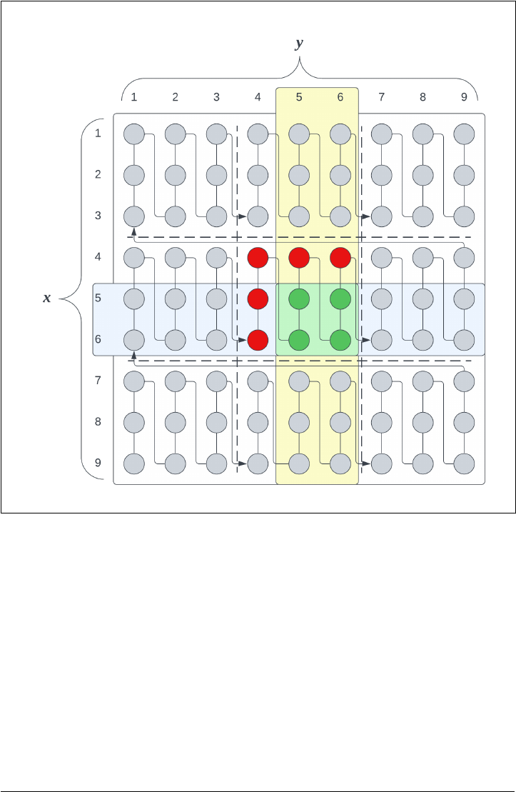
Figure 6-4. Using a space-lling curve like a z-order curve reduces the number of les

and unneeded data reads required for operations.

After applying the clustering technique to the example you only have to read a single

file. This is partly why z-ordering goes alongside an optimize action. The data needs

to be sorted and arranged according to the clusters. You might wonder if you still

need to partition the data in these cases since the data is organized efficiently. The

short answer is “yes” as you may still want to partition the data, for example, in cases

where you are not using liquid clustering and might run into concurrency issues.

When the data is partitioned optimize and zorder will only cluster and compact data

already co-located within the same partition. In other words, clusters will only be

created within the scope of data inside a single partition, so the benefits of zorder still

directly rely on a good choice of partitioning scheme.

Performance Considerations | 159

11 There is a version of this written in Python to encourage additional exploration in the Chapter 12 section of

the book repository.

The method for determining the closeness, or cluster membership, relies on inter‐

leaving the column bits and then range partitioning the dataset.

You can use these steps to accomplish this:

1. Create columns containing the coordinate positions as integers.1.

2. Map them to binary values.2.

Bitwise interleave the binary values.

4. Map the resulting binary values back to integers.4.

5. Range partition the new 1-dimensional column.5.

Plot the points by coordinates and bin identifier.

160 | Chapter 6: Performance Tuning: Optimizing Your Data Pipelines with Delta Lake

12 For more technical details refer to Mohamed F. Mokbel, Walid G. Aref, and Ibrahim Kamel. 2002. Perfor‐

mance of multi-dimensional space-filling curves. In Proceedings of the 10th ACM international symposium

on Advances in geographic information systems (GIS ’02). Association for Computing Machinery, New York,

NY, USA, 149–154. https://doi.org/10.1145/585147.585179

Figure 6-5. Showing the results of a calculation to produce z-ordered clusters.

The results are shown in Figure 6-5. They don’t quite show the same behavior as

Figure 6-4 which is very neat and orderly, but it does clearly show that even with a

self-generated and directly calculated approach you could create your own zordering

on a dataset. From a mathematical perspective, there are more details and even

enhancements that could be considered but this algorithm is already built into Delta

Lake so for the sake of our sanity this is the current limit of our rigor.

Performance Considerations | 161

13 This example comes from a fuller walkthrough highlighting how liquid clustering works to both split

apart larger partitions as well as to coalesce smaller ones, for the full example check out https://denny

glee.com/2024/02/06/how-delta-lake-liquid-clustering-conceptually-works/

More recently there have been questions about whether any table ought to be par‐

titioned so that there are fewer constraints on the further development of ideas

like z-ordering. This is partly because it can be very difficult to settle on the right

partitioning columns from the outset outside of highly static processes. Needs can

also change over time leading to added maintenance work in updating the table

structure (see the example if you need to do this). One development in this area may

reduce these maintenance burdens and decisions for good.

Cluster By

The end of partitioning? That’s the idea. The newest and best-performing method for

taking advantage of data skipping came in Delta Lake 3.0. Liquid clustering takes the

place of traditional hive-style partitioning with the introduction of the cluster by

parameter during table creation. Like zorder, cluster by uses a space-filling curve

to determine the best data layout but changes to other curve types that yield more

efficiency. Figure 6-6 shows how different partitions may either get coalesced together

or broken down in different combinations within the same table structure.

Figure 6-6. An example le layout resulting from applying liquid clustering on a data‐

set.

162 | Chapter 6: Performance Tuning: Optimizing Your Data Pipelines with Delta Lake

Where it starts to get different is in how you use it. Liquid clustering must be declared

during table creation to enable it and is incompatible with partitioning, so you can’t

define both. When set it creates a table property, clusteringColumns, which can be

used to validate liquid clustering is in effect for the table. Functionally, it operates

similarly to zorder by in that it still helps to know which columns might yield the

greatest filtering behaviors on queries, so you should still make sure to keep our

optimization goals in sight.

You also will not be able to zorder the table independently as the action takes place

primarily during compaction operations. A small side benefit worth mentioning is

that it reduces the specific information needed to run optimize against a set of tables

because there are no extra parameters to set, allowing you to even loop through a list

of tables to run optimize without worrying about matching up the correct clustering

keys for each table. You also get row-level concurrency, which is a must-have feature

for a partitionless table, which means that most of the time you can stop trying to

schedule processes around one another and reduce downtime since even optimize

can be run during write operations. The only conflicts that happen are when two

operations try to modify the same row at the same time.

File clustering, like the one shown in Figure 6-6, gets applied to compaction in

two different ways. For normal optimize operations it will check for changes to the

layout distribution and adjust if needed. This newer clustering enables a best-effort

application of clustering the data during write processes which makes it far more

reliably incremental to apply. This means less work is required to rewrite files during

compaction which also makes that process more efficient as well. This feature is

called eager clustering. This means that for data under the threshold (512GB by

default), new data appended to the table will be partially clustered at the time of the

write (the best effort part). In some cases, the size of these will vary from the larger

table until a larger amount of data accumulates and optimize is run again. This is

because the file sizes are still driven by the optimize command.

To use the cluster by argument you need at least a writer version

of 7 in a Delta Lake release with the liquid clustering table feature

present and enabled. To only consume the tables you need a reader

version of 3. This means that if you have other/older consumers

in the environment you are at risk of breaking workflows while

migrating to newer versions and protocols.

Explanation

Cluster by uses a different space-filling curve than zorder but without the presence

of partitions it creates clusters across the whole table. Using it is fairly straightforward

as you simply include a cluster by argument as a part of your table creation

statement. You must do so at creation or the table will not be compatible as a liquid

Performance Considerations | 163

partitioning table, it cannot be added afterward. You can, however, later update the

columns chosen for the operation or even remove all columns from the clustering

by using an alter table statement and cluster by none for the latter case (there’s

an example of this soon). This means you gain great flexibility with clustering keys

because they can be changed as needs arise or consumption patterns evolve.

As you’re creating tables that are optimized for either the downstream consumers or

for your write process this presents an area where you can make just such a decision

between the two. Similar to other cases, if the goal is to get the speediest write perfor‐

mance then you can elect not to include any clustering at all or as little as you wish.

For the downstream consumers though you gain a considerable advantage. You saw

in Chapter 6 that although it’s possible to re-partition a given table, it’s not the most

straightforward operation. Now you can adapt to downstream consumer needs more

optimally by redefining the clustering columns and this will be picked up during the

next compaction process to apply the layout to the underlying files. This means that

as usage patterns change, or even if you made questionable assumptions or errors

in your original layout, they become more easily rectifiable. The following examples

show how you can leverage liquid clustering in the Databricks environment.

If the initial write to a table is larger than 10TB, for example, if

you use a CTAS (Create Table As Select) statement to do a one-

time conversion, the first compaction operation can suffer from

performance issues and take some time to complete. The clustering

quality may also be affected somewhat. It is recommended to run

the process in batches for large tables as a result but otherwise,

even tables of 100TB can have liquid clustering applied to them.

Hopefully, it has become apparent that liquid clustering offers several advantages over

hive-style partitioning and zordering tables whenever it’s a good fit. You get faster

write operations with similar read performance to other well-tuned tables. You can

avoid problems with partitioning, You get more consistent file sizes which makes

downstream processes more resistant to task skewing. Any column can be a cluster‐

ing column and you gain much more flexibility to shift these keys as required. Lastly,

thanks to row-level concurrency, conflicts with processes are minimized allowing

workflows to be more dynamic and adaptable.

Examples

In this example, you’ll see the Wikipedia articles dataset found in the /databricks-

datasets/ directory available in any Databricks workspace. This parquet directory

has roughly 11GB of data (disk size) across almost 1100 gzipped files.

Start by creating a DataFrame to work with and add a regular date column to the set

then create a temporary view to work with in SQL afterward.

164 | Chapter 6: Performance Tuning: Optimizing Your Data Pipelines with Delta Lake

## Python

articles _path = (

“/databricks-datasets/wikipedia-datasets/” +

“data-001/en_wikipedia/articles-only-parquet”)

parquetDf = (

spark

.read

.parquet(articles_path)

)

parquetDf.createOrReplaceTempView("source_view")

With a temporary view in place to read from then to create a table you can simply

add the cluster by argument to a regular CTAS statement to define the table.

## SQL

create table

example.wikipages

cluster by

(id)

as (select *,

date(revisionTimestamp) as articleDate

from source_view

)

Now you still have a normal statistics collection action to think about so you probably

want to exclude the actual article text from that process, but you also created the

articleDate column which you probably want to use for clustering. To do this you

can add the three following steps: reduce the number of columns you collect statistics

on to only the first 5, move both the articleDate and text columns, and then finally

define the new cluster by column. You can do all of these using alter table

statements.

## SQL

ALTER TABLE example.wikipages set tblproperties ("delta.dataSkippingNumIndexed

Cols"=5);

ALTER TABLE example.wikipages CHANGE articleDate first;

ALTER TABLE example.wikipages CHANGE `text` after revisionTimestamp;

ALTER TABLE example.wikipages CLUSTER BY (articleDate);

After this step, you can run your optimize command and everything else will be

handled for you. Then you can use a simple query like this one for testing:

## SQL

select

year(articleDate) as PublishingYear,

count(distinct title) as Articles

from

example.wikipages

where

month(articleDate)=3

Performance Considerations | 165

14 If you wish to dive more deeply into the mechanisms and calculations used to create bloom filter indexes

consider starting here: https://en.wikipedia.org/wiki/Bloom_lter.

and

day(articleDate)=4

group by

year(articleDate)

order by

publishingYear

Overall the process was easy and the performance was comparable, only slightly

faster than the zordered Delta Lake table. The initial write for liquid partitioning also

took about the same amount of time. These results should be expected because the

arrangement is still basically linear. One of the biggest gains in value here, however,

is the added flexibility. If at some point you decide to revert to clustering by the

id column as in the original definition, you just need to run another alter table

statement and then plan for a bigger-than-usual optimize process later on. Whether

you end up using liquid clustering or rely on the familiar z-ordering, there’s still

an additional indexing tool you can put in place that further improves the query

performance of chosen tables.

Bloom Filter Index

A bloom filter index is a hashmap index that identifies whether or not a value

probably exists in a file or definitely does not.

They are considered space efficient

because an index file containing the hashed value (in a single row) is stored alongside

the associated data file, and you can specify which columns you wish to be indexed.

The catch is that you want to have a reasonable idea of how many distinct values

need to be indexed because this will determine the length of hashes needed to avoid

collisions if it is set too small or to avoid wasting space if it is set too large.

Bloom filter indexes can be used by either parquet or Delta Lake tables in Apache

Spark even if they use liquid clustering. At runtime, Spark checks for the existence of

the directory and uses the index if it exists. It does not need to be specified during

query time.

A Deeper Look

A bloom filter index is created at the time of writing files, so this has some implica‐

tions to consider if you want to use the option. In particular, if you want all of the

data indexed then you should define the index immediately after defining a table but

before you write any data into it. The trick to this part is defining the index correctly

requires you to know the number of distinct values of any columns you want to

index ahead of time. This may require some additional processing overhead, but for

the example, you can add a count distinct statement and get the value as part of

166 | Chapter 6: Performance Tuning: Optimizing Your Data Pipelines with Delta Lake

the process to accomplish this using only metadata (another Delta Lake benefit). Use

the same table from the cluster by example but now insert a bloom filter creation

process right after the the table definition statement (before you run the optimize

process).

## Python

from pyspark.sql.functions import countDistinct

cdf = spark.table("example.wikipages")

raw_items = cdf.agg(countDistinct(cdf.id)).collect()[0][0]

num_items = int(raw_items * 1.25)

spark.sql(f"""

create bloomfilter index

on table

example.wikipages

for columns

(id options (fpp=0.05, numItems={num_items}))

""")

Here the previously created table is loaded and you can bring in the Spark SQL

function countDistinct to get the number of items for the column you want to

add an index for. Since this number determines the overall hash length it’s probably

a good idea to pad it, like where raw_items is multiplied by 1.25 there was an

additional 25% added to get num_items, to allow for some growth to the table (adjust

according to your projected needs). Then define the bloom filter index itself using

SQL. Note that the syntax of the creation statement details exactly what you wish to

do for the table and is pretty straightforward. Then specify the column(s) to index

and set a value for fpp (more details are in the configuration section) and the number

of distinct items you want to be able to index (as already calculated).

Conguration

The fpp value in the parameters is short for false positive probability. This number

sets a limit on what rate of false positives is acceptable during reads. A lower value

increases the accuracy of the index but takes a little bit of a performance hit. This is

because the fpp value determines how many bits are required for each element to be

stored so increasing the accuracy increases the size of the index itself.

The less commonly used configuration option, maxExpectedFpp, is a threshold value

set to 1.0 by default, which disables it. Setting any other value in the interval [0,

1) sets the maximum expected false positive probability. If the calculated fpp value

exceeds the threshold the filter is deemed to be more costly to use than it is beneficial

and so is not written to disk. Reads on the associated data file would then fall back to

normal Spark operation since no index remains for it.

Performance Considerations | 167

You can define a bloom filter index on numeric types, datetime types, strings, and

bytes but you cannot use them on nested columns. The filtering actions that work

with these columns are: and, or, in, equals, and equalsnullsafe. One additional

limitation is that null values are not indexed in the process so filtering actions related

to null values will still require a metadata or file scan.

Conclusion

When you set out to refine the way you engineer data tables and pipelines with

Delta Lake, you may have a clear optimization target, or you might have conflicting

objectives. In this chapter, you saw how partitioning and file sizes influence the

statistics generated for Delta Lake tables. Further, you saw how compaction and

space-filling curves can influence those statistics. In any case, you should be well

equipped with knowledge about the different kinds of optimization tools you have

available to you in working with Delta Lake. Most specifically, note that file statistics

and data skipping are probably the most valuable tools for improving downstream

query performance and you have many levers you can use to impact those statistics

and optimize for any situation. Wherever your goal is this should prove to be a

valuable reference as you evaluate and design data processes with Delta Lake.

168 | Chapter 6: Performance Tuning: Optimizing Your Data Pipelines with Delta Lake

CHAPTER 7

Successful Design Patterns

A Note for Early Release Readers

With Early Release ebooks, you get books in their earliest form—the author’s raw and

unedited content as they write—so you can take advantage of these technologies long

before the official release of these titles.

This will be the 13th chapter of the final book. Please note that the GitHub repo will

be made active later on.

If you have comments about how we might improve the content and/or examples in

this book, or if you notice missing material within this chapter, please reach out to the

editor at gobrien@oreilly.com.

With the flexibility and applicability of Delta Lake to data applications, trying to

capture all of the cases for which you can use it is like trying to describe all of the

potential uses of paper. The variety feels limitless and its value is legion. That being

said, we do our best to capture exemplary cases highlighting some great uses of Delta

Lake and the value in doing so.

We will start by showing how the performance optimizations and simplified mainte‐

nance operations in Delta Lake helped Comcast slash the amount of resources they

needed to run their smart remote process by 10x. We then describe how Scribd

helped evolve the Delta Lake landscape and created the Delta Rust implementation,

which is 100x cheaper than the equivalent structured streaming applications. Finally,

we see how Delta Lake feeds high-volume operational CDC ingestion and supports

real-time workloads from Flink at DoorDash, creating a single source of truth lake‐

house from many different operational systems. Each section is accompanied by

169

several resources you may wish to review to further explore the stories found here in

greater detail.

Slashing Compute Costs

The focus of this section reaches many audiences, literally! It’s no secret that there

has been somewhat of an eruption in the number of streaming entertainment services

over the last several years. Organizations supporting these kinds of services tend to

have large volumes of high throughput streaming data that they need to manage to

help support the service.

High-Speed Solutions

Streaming media services usually capture data from individual end-user devices

which includes several different components. To run such services successfully you

may require varying kinds of information about device health, application status,

playback event information, and interaction information. This usually translates to a

need for building high-throughput stream processing applications and solutions.

One of the most critical components in these streaming applications is ensuring the

capture of the data with reliability and efficiency. In Chapter 9 several implementa‐

tion methods and their benefits demonstrate how Delta Lake can play a critical role

in doing exactly these kinds of data capture tasks. Delta Lake is often the destination

for many of these ingestion processes because it has ACID transaction guarantees and

additional features like optimized writes that make high-volume stream processing

better and easier.

Let’s say you want to monitor the Quality of Service (QoS) across all of your users

in near real-time. To accomplish this task you usually need not just playback event

information, but also the relevant context from each user’s session, a sequence of

interactions bound together over some timespan. Sessionization is often an important

cornerstone to many downstream operations beyond ingestion and typically falls into

the data engineering stages of a larger data process as shown in Figure 7-1. With

session information and other system information in Delta Lake, you can power

downstream analytics use cases like quality of service measurement or trending item

recommendations while maintaining a low turnaround time in processing.

170 | Chapter 7: Successful Design Patterns

1 For an extended exploration of a QoS solution end-to-end we suggest this blog with accompanying notebooks

from Databricks: https://www.databricks.com/blog/2020/05/06/how-to-build-a-quality-of-service-qos-analytics-

solution-for-streaming-video-services.html.

2 “Winning the Audience with AI: How Comcast Built An Agile Data And Ai Platform At Scale | (Comcast)”.

Spark + AI Summit 2019. Accessed Nov. 6 2023 https://www.youtube.com/watch?v=5sDH_dJqoYo

Figure 7-1. A reference architecture for Quality of Service monitoring with Delta Lake.

Building out these pipelines is often fairly complex and will involve the interaction

of multiple pipelines and processes. At the core, you will find that each component

boils down to the idea of needing to build a robust data processing pipeline to serve

multiple business needs.

Smart Device Integration

Comcast developed a successful smart remote control device to change the way peo‐

ple watch television. The crux of the data problem they had is that this kind of system

requires large amounts of data processing and several technical and organizational

challenges. Through the use of Delta Lake as a data format, many of these challenges

were overcome and they were able to slash their cloud infrastructure requirements,

for one of their most critical workloads, by 90%. They were also able to solve many

quality-of-life issues around these data processes. Here you can see how they solved

many of those challenges.

Comcast’s Smart Remote

Comcast is the largest American multinational telecommunications and media con‐

glomerate, and here you can see how they were able to drastically reduce the amount

of cloud resources required to run their most important workloads.

Comcast has

strived toward changing how people interact with their televisions through their

voice remote which acts as a central point of access. So, as you might expect, there are

Slashing Compute Costs | 171

a lot of critical data workloads that center around the device at the edge. Figure 7-2

shows a high-level example of the interaction flow.

Figure 7-2. Comcast’s smart remote control provides an alternative interface for enter‐

tainment.

Before exploring how they’re building their solutions on Delta Lake, it might be

useful to review more specific information about the scale of their operations. Com‐

cast drives interactions through the Xfinity(R) smart remote and their customers

used this remote 14 billion times in 2018-2019 (Figure 7-3 illustrates the relative

scale to data processing). Users expect many things in their experience with the

applications like accurate searches and feeling enabled to find the right content for

consumption. The user’s experience should also have elements of personalization that

make the experience their own. With the voice remote users can interact with the

whole system; anything is just a quick phrase away. On top of this, they use user data

to create personalized experiences.

Consider the technical components essential to running such services behind the

scenes. First, receiving voice commands as input (something that’s exploded in popu‐

larity more recently) is a technically challenging problem. There’s the transformation

of voice to a digital signal which then has to be mapped to each needed command.

There’s often an additional component to this mapping of correcting for intent. Is

it more likely for someone to search for a show called “How It’s Made” or are they

asking about other shows about how some particular thing is made? If it is a search

command there is still a need to find similar content through a matching algorithm.

All of this gets wrapped together into a single interface point in a setting where the

user experience needs to be measured against accuracy so getting bits of data about

172 | Chapter 7: Successful Design Patterns

3 For a more robust treatment of embeddings see, e.g. Marcos Garcia; Embeddings in Natural Language

Processing: Theory and Advances in Vector Representations of Meaning. Computational Linguistics 2021; 47

(3): 699–701. doi: https://doi.org/10.1162/coli_r_00410

these processes and enabling analytics to assess immediate problems or long-term

trends is also critical.

So now we have voice inputs that have to be converted to embedding vectors (vectors

of numeric data capturing semantic meaning as “tokens”) as well as contextual data

(this could be what type of page the user is on, other recent searches, date-time

parameters, etc.) for each interaction with the remote.

The goal is to collect all this

and provide inference back through the user interface (UI) in nearly real-time. From

a functional standpoint, there’s also a large amount of telemetry information that

needs to be collected to maintain insights into things like device health, connectivity

status, viewing session data, and other similar concerns.

Once the problem of getting this data from individual devices to a centralized

processing platform is solved there are still additional challenges in deciding how

to standardize the data sources as multiple versions of devices may have differing

available information or usage regions may have differing collection laws that mean

fuller or lesser contents of captured events. Downstream from standardization, there

is still a need to organize the data and create actionable steps in a fit-for-function

format.

Expecting all of this to happen from a single team would require a huge amount

of effort and a lengthy amount of time so enabling multiple teams to collaborate to

tackle the complexity would be beneficial if not an absolute necessity.

Earlier Attempts

To support the voice remote Comcast needed to be able to analyze queries and look

at user journeys to do things like measure the intention of a query. At a rate of up to

15 million transactions per second, Comcast needed to enable sessionization across

billions of sessions on multiple Petabytes of data. Running on native AWS services

they would overrun limits and increase the concurrency they were using until they

were eventually running 32 concurrent job runs across 640 virtual machines to be

able to get to the scale they needed for sessionization. The processing flow is shown

in Figure 7-3. This led them to seek a scalable, reliable, and performant solution.

Slashing Compute Costs | 173

Figure 7-3. To scale the earlier data ingestion pipeline Comcast had to crank up the

concurrency.

Delta Lake Reduces the Complexity

Delta Lake was built to help solve exactly these kinds of problems. ACID transactions

and support for multiple writers with features like optimized writes and autocompac‐

tion each play a role in simplifying and overcoming the challenges involved with

large-scale stream processing tasks. Enabling additional features like delta.randomFi

lePrefixes for high transaction rates with cloud providers allows you as an engineer

to achieve massive scale with optimal efficiency. By making this change Comcast was

able to run the same ingestion process with a single Spark job on just 64 virtual

machines. The resulting process flow is shown in Figure 7-4.

174 | Chapter 7: Successful Design Patterns

Figure 7-4. Delta Lake provides the foundation for optimized ingestion and sessioniza‐

tion.

If this was the whole story you would probably already be convinced of the value

Delta Lake can bring to ease processing burdens. What’s great is that’s not the whole

story. In their Databricks environment, Comcast was able to readily access this

sessionized data for multiple downstream purposes.

It was mentioned already that in building a process like this different kinds of

machine learning tasks like the creation of embedding vectors or model inference

may be involved. In particular, there would be a need to transform that voice input

into meaningful action. By capturing the sessionized data and storing it efficiently,

data scientists can build modeling pipelines quickly and easily.

MLflow, another open-source product, offers many features for

improving the end-to-end MLOps process. Some of MLflow’s key

features include tracking and comparing multiple model versions

in experiments, a registry for management, and mechanisms ena‐

bling the easier deployment of model objects. This also includes

specific support for Large Language Models (LLMs) through some

of the more recently added features.

Since Comcast is using MLFlow they get additional side benefits from Delta Lake

in their machine learning processes. With the data source tracking available in the

Slashing Compute Costs | 175

4 To compare the entire capabilities for tracking different kinds of files in MLflow experiments we

suggest this section of their documentation: https://mlflow.org/docs/latest/python_api/mlflow.data.html?high

light=delta#mlow-data

experiment for a project MLflow can track information about the Delta Lake table

being used for the experiment without having to make a copy of the data in the

same way as you would with a CSV file or other data sources.

Since Delta Lake

also has time travel capabilities, machine learning experiments can have enhanced

reproducibility which would benefit anyone maintaining data science products in

production.

Figure 7-5. Delta Lake helps enable reliable end-to-end MLOps processes.

Another important target is to be able to monitor the telemetry data involved for

QoS or other similar types of analytical applications. In Comcast’s case, they used

Databricks SQL to run analytical workloads directly on their Delta Lake tables instead

of in Redshift as they had previously. They reported for a pilot of this approach they

chose their 10 worst performing queries to evaluate the performance. They observed

a huge reduction in query runtime latency of over 70%.

176 | Chapter 7: Successful Design Patterns

Figure 7-6. Performance comparison results for query running times in Databricks SQL

on Delta Lake vs Redshi.

In the end, it’s looking to be highly advantageous for Comcast to continue innovating

with Delta Lake. They’ve so far experienced huge savings gains in their data ingestion

processes and have a promising outlook on improving reporting. Overall this should

allow them to improve end-user experiences for their smart remotes further and

increase overall satisfaction rates.

Ecient Streaming Ingestion

Suppose you have some large ingestion pipelines running on Kafka and Databricks to

feed your Delta Lake environment. Now suppose you have a crack engineering team

that decides to invest significant efforts into reducing costs by crafting a solution for

small streams that don’t require the heavy-lifting capabilities of Spark. You also want

to bring all of that data together downstream from those ingestion processes. What

you might be looking for then is something like the team at Scribd has done.

Streaming Ingestion

Stream processing applications for ingestion tasks are relatively common. We have

a large array of streaming frameworks out there to choose from. Among the most

common ones are the open-source Apache Kafka, Kinesis from AWS, Event Hubs

in Azure, and Google’s Pub/Sub. One reason for this is a general trend towards

streaming data applications.

While there is certainly a wide variety of applicability covering interesting subjects

like real-time telemetry monitoring of IoT devices and fraudulent transaction moni‐

toring or alerting, one of the most common cases for stream processing is large-scale

Ecient Streaming Ingestion | 177

5 Many teams document their own journey of landing streaming data sources in Delta Lake, for example, the

Michelin team captured a step-by-step implementation guide to building a Kafka+Avro+Spark+Delta Lake

in a Microsoft Azure environment: https://blogit.michelin.io/kaa-to-delta-lake-using-apache-spark-streaming-

avro/

6 Architecture diagram comes from this Databricks blog post accessed 2023-12-07: https://www.databricks.com/

blog/2022/09/12/simplifying-streaming-data-ingestion-delta-lake.html

Our use here of the term “artificial intelligence” is used in the classical software development sense of

narrow AI meaning the application of machine learning algorithms to make automated business decisions

without human interaction, see e.g. https://hai.stanford.edu/sites/default/les/2023-03/AI-Key-Terms-Glossary-

Denition.pdf.

Refer to the section on the medallion architecture in Chapter 11 or Chapter 9 for more details on implement‐

ing stream processing applications and Delta Lake.

and dynamic data ingestion.

For many organizations collecting data about activi‐

ties by end-users on mobile applications or point-of-sale (POS) data from retailers

directly translates to success in supporting mission-critical business analytics applica‐

tions. Acquiring large amounts of data from widely dispersed sources quickly and

correctly allows businesses to become more rapidly adaptable to changing conditions

as well (Figure 7-7 shows a unified architecture across many streaming sources).

Figure 7-7. An example reference architecture diagram for stream processing applica‐

tions with a Delta Lake sink from Databricks.

Great flexibility, through the enablement of real-time processes and the use of artifi‐

cial intelligence applications, is fueled by dynamic and resilient data pipelines often

falling into this category.

In all of these, there’s usually an element of capturing

inbound data for later analytical or evaluation purposes, so while there might be

additional components in some processing pipelines at the end of the day this process

applies to most stream processing applications.

178 | Chapter 7: Successful Design Patterns

Figure 7-8. A simplied streaming data ingestion architecture for IoT devices specic to

Kaa

Consider the case of IoT data coming in from devices. If you send all the data into

Kafka you can build a Spark application to consume that stream and capture all of the

original data as it is received following the model of the medallion architecture. Then

you can create business-level reporting and send those results out to be consumed in

a downstream application. Naturally, there are many variations on this approach, but

the general pipeline model is similar. At Scribd, this application was so common they

built a new framework around implementing this process.

The Inception of Delta Rust

While it started as an open publishing platform, now Scribd is a digital document

library, with over 170M documents in over 150 categories and counting. Part of their

mission is to change the way the world reads. They aim to do so by providing a wide

range of reading material at a fair price for both creators and consumers, providing

intellectual property protection for creators and keeping costs low, preferring to build

their brand on community rather than advertising.

Inherent to its existence as a digital library, Scribd runs its website as well as

mobile applications. Users can use Scribd’s website and mobile applications to browse

through a digital library with millions of presentations, research papers, templates,

and many other kinds of documents. All of the documents in the library are uploa‐

ded by creators, writers, and editors using multiple common document formats

like .pdf, .txt, .doc, .ppt, .xls, and .docx. There is also a subscription system. All of

these different system components translate to events that have to be collected and

handled accordingly. At Scribd, they accomplish this using a fairly large number of

event streams through Kafka.

Ecient Streaming Ingestion | 179

Building a streaming ingestion pipeline typically requires multiple components.

Putting this into the immediate context a straightforward design approach would

be to build a stream processing application for each topic stream coming from

Kafka. In the case of Scribd, we can easily build a list of some of the probable event

topic streams: creator uploads, reading events, system log-in or authentication events,

subscription events, web traffic events, searches, item bookmarking or saving events,

and item sharing events. This means many different stream processing applications

will be involved which usually leads to the development of some kind of framework

to reduce development and maintenance overhead across all the applications.

Maintaining a stream processing framework for many event streams can be quite a

complex task, and, without careful planning, quite expensive as well. Here is the story

of the evolution of Scribd’s stream processing framework leading up to their creation

of the kafka-delta-ingest library and how they cut their ingestion costs by 95%.

Evolution of Ingestion

The stream processing platform at Scribd has been revamped a couple of different

times. Early on all the processing was done in Kafka and Hadoop, which used to be

a fairly standard stream processing approach. This version of the platform was later

subsumed by a move to Kafka and Databricks using Spark Structured Streaming and

Delta Lake. This was a favorable move for Scribd, partly because of Delta Lake’s fea‐

tures, like the optimize and vacuum utilities and the addition of ACID transactions.

However, in Scribd’s case, there were many topic streams and many of them were

also on the small side. This led to some attempts to reduce spiraling ingestion costs.

One natural approach is to stack multiple stream processing applications on the same

cluster. This allows you to make use of cluster resources more optimally. At Scribd,

larger dedicated clusters were still used “when it didn’t seem wasteful” to do so,

i.e. when there were large tasks that efficiently utilized the cluster resources. Many

small streams were instead stacked (run simultaneously on the same cluster) which

produces a similar level of efficient resource utilization and thus reduces overall pro‐

cessing costs. There are still some challenges in doing this though. Making decisions

about how to logically group topics can be frustrating. There’s always the possibility

that one of the processing tasks could fail, causing all the stacked streams on that

cluster to subsequently fail. This is in addition to the already slightly challenging task

of trying to accommodate maintenance tasks in your ingestion processes.

The Scribd team had a few desires for improving the situation:

• further reducing the costs if possible•

•

different observability of the ingestion processes

•

• better handling of job failures•

180 | Chapter 7: Successful Design Patterns

• more flexible adjustment to changes in the throughput size of event streams•

This also led to thoughtful reflection on how they might approach the problem.

Would it be possible to do this without Spark or find some more minimal overhead

method? How would they still maintain their standardization on Delta Lake since it

made stewardship so much easier?

To the Scribd team at the time, it seemed like with some invested effort, there

might be another way to approach the problem. They have relatively simple ingestion

processes that are append-only operations with no filters, joins, or aggregations and

only use a subset of Delta Lake’s features, which proved to simplify the development

of an alternative.

The scenario at Scribd led to their investment in developing two projects that are

now well-supported and accepted parts of the larger Delta Lake ecosystem. The

first project is delta-rs, the Rust-based implementation of the Delta Lake protocol

explored in depth in Chapter 5. The second project is kafka-delta-ingest, a light‐

weight companion framework designed to quickly and easily ingest data from a Kafka

topic stream into a Delta Lake table. Together they form an efficient operating pair

(Figure 7-9 shows the simplified data flow).

Figure 7-9. Scribd’s kafka-delta-ingest in tandem with delta-rs for ecient inges‐

tion.

Undertaking such an endeavor was not without risks or potentially blocking issues.

The risk of corrupting the delta log posed one challenge, as did the need to manually

control offset tracking in Kafka to avoid duplicate or dropped records. They also need

Ecient Streaming Ingestion | 181

9 Some of these S3 issues are discussed in the D3L2 web series episode “The Inception of Delta Rust” on

Youtube: https://www.youtube.com/watch?v=2jgfpJD5D6U.

10 AWS r5 type metrics can be found here: https://aws.amazon.com/ec2/instance-types/r5/

to support multiple writers, and some limitations in AWS S3 require specific handling

(e.g. S3 lock coordination).

Scribd runs anywhere from 70-90 of these kafka-delta-ingest and delta-rs pipe‐

lines in production. They run serverless computation of these pipelines through AWS

Fargate and monitor everything in Datadog. Some of the things they monitor include

message deserialization logs and several metrics: the number of transformations,

failures, the number of arrow batches in memory, the sizes of parquet data files

written, and the current time lag in Kafka streams.

Figure 7-10. Some of the cost-saving examples Scribd shared during Data+AI Summit

2022 where they compare the cost of running a process originally in Spark and then

similarly using delta-rs. e Rust resources show vCPUs and memory allocation whereas

the Spark clusters use entire EC2 instances, r5.large instances as shown each has 2

vCPUs and 16GB RAM.

All of this led to rather significant cost savings in ingestion processing as with the

tools the Scribd team built the cost for running some of the stream processing

applications is reduced to as little as 100 times lower. Another feature that rounds out

this fantastic achievement is that this is accomplished in such a way (by remaining

standardized on Delta Lake) that the ingested data is immediately available for analyt‐

182 | Chapter 7: Successful Design Patterns

ics and machine learning processes or further integration with other batch processes

in their Databricks environment and it maintains queryability.

Coordinating Complex Systems

From smart devices and entertainment to security and digital payment systems, there

is no shortage of high-volume data sources. With Scribd, much of the focus was

on simple event capture with less stress on the operational systems where kafka-delta-

ingest is a viable solution. Now let’s consider cases where the edge of interaction

with the outside world is less straightforward and requires more services. It’s more

messy and more human. Complex applications that continuously evolve tend to have

many more integrated operational components that need to stay in harmony over

time or you might find yourself spending more time curating existing data instead

of thinking about new requirements, sources, or processes as you would probably

prefer.

Figure 7-11. Retail merchant credit transactions present just one area where we might

see complex system interactions.

The inclusion of multiple, real-time, operational databases and the demand for gener‐

ating business value often means that the information from those databases needs

to be collected into a unified location for the development of analytics and machine

learning applications. Other systems may not have operational databases but rely on

event-driven systems. Oftentimes this data will be needed in conjunction with data

from other systems creating a relatively complex data ecosystem, like customer trans‐

action data with anonymized trend data available on the open market for example.

Figure 7-11 shows how you combine data sources such as these to support multiple

downstream applications. Relying on a lakehouse format like Delta Lake with its

broad array of connectors for different systems reduces this complexity and enables

analytical and artificial intelligence-based applications.

Coordinating Complex Systems | 183

11 If you want to spend more time exploring CDC, also known as logical log replication, we suggest Designing

Data Intensive Applications by Martin Kleppmann (O’Reilly).

Combining Operational Data Stores at Doordash

Many people have found themselves in situations where it would be convenient

if someone could help them pick up meals, groceries, electronics, or pretty much

anything else for them and maybe save themselves a trip out. DoorDash helps to

fill all kinds of needs by providing flexibility and convenience through their delivery

services. While most are familiar with their “gig” based operating methodology, it

may be helpful to note a couple of particular points to consider.

There are multiple parties involved in the purchase process through DoorDash.

Typically there are the requesters, people who make deliveries, and restaurants or

merchants who will prepare orders or make products available. Without even step‐

ping into the larger IT ecosystem of the DoorDash organization there is already an

apparent need for large-scale low-latency data pipelines, i.e. streaming data applica‐

tions because each “event” itself is a collation of many events as it steps through the

process.

DoorDash is leveraging Delta Lake as part of its data ecosystem in two ways. The

first is to simplify the management of large-scale Change Data Capture (CDC)

and downstream exposure of data for analytics. The second is supporting real-time

workloads in Flink. Both capture some of the benefits of utilizing Delta Lake in your

architectural designs.

Change Data Capture

Change Data Capture, or CDC, is a common application pattern that often needs to

be supported for a variety of reasons.

At DoorDash they use CDC for replication

of operational databases supporting multiple services into the analytical environment.

This is driven by a historical need to be able to answer a question: “How many orders

did DoorDash do yesterday?” Earlier on this was an easier task as the solution to

answering the question could be accomplished by creating a copy of the database and

using queries against the copy to answer analytical questions or perform data science

tasks.

As DoorDash grew their service architecture evolved leading to an environment with

multiple operational databases that also come in multiple flavors like CockroachDB,

PostgreSQL, and Apache Cassandra. Seeking to get data from these databases in

the simplest way they initially got snapshots from the databases and pulled them in

daily. While this approach worked it did pose problems, specifically tracking data

versioning and a need to filter the snapshots to incrementalize the data process

184 | Chapter 7: Successful Design Patterns

efficiently. After trying various changes in the environment the team eventually set

out to develop a more robust system.

The key system requirements for our purpose were:

• Less than a day of data latency•

• Use a Lakehouse design pattern•

•

Support schema evolution

•

• Allow for data backfilling•

• Enable analytical workloads•

•

Write once read many times

•

• Avoid late-arriving data•

• Build with open-source software•

The design that arose from these requirements is a streaming CDC framework built

on Spark Structured Streaming that replicates change feeds into a unified source of

truth built on Delta Lake that supports downstream integrations across a wide range

of query interfaces. Features like merge support and ACID transactions helped make

Delta Lake a critical component of the design.

Figure 7-12. e design of DoorDash’s CDC-enabled Lakehouse architecture.

Coordinating Complex Systems | 185

The success of this design could be measured in many ways but there are several the

team highlights. The system supports 450 streams (one-to-one with tables) running

24/7 on over 1000 EC2 nodes. This translates to about 800GB ingested daily from

Kafka with a total daily processing volume of about 80TB. The design far exceeded

the initial requirements and attained a data freshness of less than 30 minutes. They

have enabled the self-service creation of tables for data users in the environment

which become available in less than an hour.

Delta and Flink in Harmony

With real-time events being of central importance to DoorDash, their heavy use

of Kafka is hardly surprising. Apache Spark is a natural choice for many stream

processing applications; however, it’s not the only choice. Some teams at DoorDash

use Apache Flink for many real-time processes, and, therefore, it should also be

easily supportable. In Chapter 5 you saw how the Flink/Delta Connector works

operationally but here it could be useful to see how this can be pulled into a larger

data ecosystem to provide both flexibility and reliability.

The real-time platform team at DoorDash is managing Petabytes of vital customer

events every day and needs to provide a platform to enable data users and applica‐

tions to capture, create, or access this information. Adding the Flink/Delta Connector

extends the number of ways that users and applications can interact with Delta Lake

which combines the fast operational nature of Flink with a storage format built to

handle exactly those kinds of workloads and provides a common format useable

across the whole data platform even while different teams choose to leverage different

application processing frameworks.

Figure 7-13. e starting state of processes at DoorDash before moving to Delta Lake.

186 | Chapter 7: Successful Design Patterns

This is exactly what this change at DoorDash enabled, easy integration with their

current tooling with the addition of ACID guarantees at massive scale. Previously

this process was taking place with regular Parquet files which adds additional com‐

plications in the form of write-locks and other challenges. Additionally, the quality

of life improvements gained through easy-to-use compaction operations and the

ability to do these operations while stream processing applications are still running is

highly valuable. As is the efficiently queryable state achieved through the inclusion of

z-ordering clusters on the data.

Figure 7-14. e resulting state of the data ecosystem at DoorDash aer moving to Delta

Lake.

The moral of the story of the DoorDash decision to adopt Delta Lake is this: even

for data systems with multiple types of tooling operating at massive scale and need

to support things like efficiently capturing data from real-time event streams or the

changes coming through operational databases Delta Lake provides reliability and

usability making it a winning choice.

Conclusion

Data applications come in many different forms and formats. Authoring those data

applications can be complex and painful. Here you’ve seen a few ways to alleviate this

pain through the many benefits of Delta Lake. In particular, the features of Delta Lake

help create a robust data environment that supports broad tooling choices, reduces

costs, and improves your quality of life as a developer.

Conclusion | 187

References

Comcast

• Transforming home entertainment with voice, data, and AI•

•

Learn the Comcast Architecture for Enterprise Metadata and Security

•

Winning the Audience with AI: How Comcast Built An Agile Data And Ai

•

Platform At Scale | (Comcast)

•

SQL Analytics Powering Telemetry Analysis at Comcast

•

Comcast makes home entertainment accessible to everyone with voice, data and

•

• SQL Analytics Powering Telemetry Analysis at Comcast•

Scribd

• Kafka to Delta Lake, as Fast as Possible•

•

Streaming Data into Delta Lake with Rust and Kafka

•

Doordash

• Writing to Delta Lake from Apache Flink•

• Apache Flink Source Connector for Delta Lake Tables•

•

Building Scalable Real-Time Event Processing with Kafka and Flink

•

• Flink + Delta: Driving Real-time Pipelines at DoorDash•

• Unlocking Near Real Time Data Replication with CDC, Apache Spark™ Stream‐•

ing, and Delta Lake

188 | Chapter 7: Successful Design Patterns

CHAPTER 8

Lakehouse Governance & Security

A Note for Early Release Readers

With Early Release ebooks, you get books in their earliest form—the author’s raw and

unedited content as they write—so you can take advantage of these technologies long

before the official release of these titles.

This will be the 14th chapter of the final book. Please note that the GitHub repo will

be made active later on.

If you have comments about how we might improve the content and/or examples in

this book, or if you notice missing material within this chapter, please reach out to the

editor at gobrien@oreilly.com.

We do many things every day without consciously thinking about them. These rote

actions, or automatic behaviors, are based on our daily routines and information

we’ve grown to trust over time. Our routines can be simple or complex, with actions

grouped and categorized into different logical buckets. Consider, for example, the

routine of locking up before leaving for the day; this is a common behavior for

mitigating risk because we simply can’t trust everyone to have our best interests in

mind. Thinking about this risk mitigation as a simple story: To prevent unauthorized

access to a physical location (entity: home, car, oce), access controls (locking mecha‐

nism) have been introduced to secure a physical space (resource) and provide authorized

admittance only when trust can be conrmed (key).

In the simplest sense, the only thing preventing intrusion is a key. While keys grant

access to a given physical space, the bearer of a given key must also know the physical

location of a protected resource; otherwise, the key has no use. This is an example

of site security, and as a mental model, it is useful when constructing a plan for the

189

layered governance and security-model for resources contained within our lakehouse.

After all, the lakehouse is only a safe space that protects what we hold near and dear if

we collectively govern the resources contained within.

But what exactly is the governance of a data resource, and how do we get started when

there are many facets of the governance landscape?

This chapter provides a foundation for architecting a scalable data governance strat‐

egy for the data assets (resources) contained within our lakehouse. We will cover

patterns for tackling challenges relating to security, privacy and governance in a

multi-tenant environment including the basics of layered security, suggested user

personas and roles (groups) as well as blueprints that can be implemented to simplify

access and authorization, audit logging, and a whole lot more. While we aim to cover

as much surface area here as possible, consider this to be a referential chapter just

scratching the surface of the myriad facets of lakehouse data governance.

Lakehouse Governance

Before diving deeper into lakehouse governance, it is important to introduce the

many facets, or components, of the governance umbrella. There are at least eight

sides to the full story, enabling us to go beyond basic access controls and stitch many

systems and services together to provide a comprehensive view over the dynamic

network of data flowing into, between, and out of our lakehouse. To kick things off,

the diagram in Figure 8-1 provides a birds-eye view of the governance components

that we’ll dive into during this chapter.

190 | Chapter 8: Lakehouse Governance & Security

Figure 8-1. Governing the lakehouse goes beyond basic le-system access controls.

There are many facets to lakehouse governance, as shown in Figure 8-1, including

the foundational components and core tenants as presented under: access controls

(1), data catalogs (2), and the elastic data management provided by the underlying

cloud-object store, or on-prem distributed file-systems (3).

Additionally, modern governance for the lakehouse also includes (4) robust auditing

across typical data management operations on a per-action basis, (5) integrated

monitoring to notify when things don’t seem right (audit), to observe and record the

objective data quality for mission-critical tables, as well as the performance of the

data pipelines, which can help surface cost-of-ownership insights as well. Connecting

the dots requires (7) data asset lineage (at least from the catalog->schema->table)

including who owns what, where, and how the data is accessed, transformed, and

otherwise “used”. Last but not least comes, (8) since the icing on the cake of all

our hard work is the ability to tie “all we know about our data” together to provide

powerful data discovery - which is arguably one of the most widespread issues given

the sprawl of data across evermore silos, platforms, and systems and services. We’ll

Lakehouse Governance | 191

get a brief overview of everything now, and then dive deeper into each of the facets of

lakehouse governance.

The Facets of Lakehouse Governance

Access Controls (1)

Provide foundational components to secure and govern the data assets within a

lakehouse through a leakproof table abstraction (no direct access to underlying

storage). Without the ability to identify a user, or service, there is no way to

approve or deny access, or authorize permissions to create, read (view), write

(insert), update (or upsert), or delete. It would be the wild west.

Data Catalogs (2)

Enable capabilities to list databases and tables, and to govern permissions at the

database, table, or column-level. The catalog provides critical metadata about

each table: defining where they reside in the data lake (delta table path in the

elastic filesystem), as well as the owner, columns, constraints, tblproperties for

each table (which we explored in Chapter 6), as well as metadata specific to the

database (dbproperties) containing a set of tables.

So access controls and data catalogs go hand-in-hand, as we can’t have one

without the other.

Elastic Data Management (3)

The last core component to the lakehouse architecture is the data lake. We

know by now that the Delta protocol aids in providing schema-enforcement and

evolution capabilities, and that by having invariants on the table level we reduce

the complexity of managing data. The data lake provides elastic scalability to

the database’s and tables contained within a data catalog, and as we will learn

soon, identity and access management plays a key role in governing data assets

securely.

Together, a strong foundational model can be constructed to power the lakehouse,

paving the way for additional critical capabilities including audit services (4) and

comprehensive monitoring (5) of access, and the generation of insights on data

operations and actions.

Audit (4)

Capturing changes in the behavior of the lakehouse, such as who, or what, has

the ability to execute specific operations (like create or delete) on resources

(catalogs, databases, tables), or when critical changes take place, like an alter

table operation on a table (recording the table version of the operation), or for

example when a table is dropped (and deleted). Simple audit also keeps track

of the access frequency to specific data assets, and tracks when something is

192 | Chapter 8: Lakehouse Governance & Security

popular, infrequently accessed, or even never accessed for read or write, or both.

We’ll cover audit trail and metrics later in the chapter.

Monitoring (5)

Capturing the behavior of the lakehouse through the lens of auditing (for security

purposes), and at the table-level (for engineers, analysts, and scientists) simply

provides a recording (timeseries) of metrics, or events. Monitoring is required

to take the metrics, and transform them to generate key performance indicators

(KPI’s), and to convert events (audit events) into metrics (KPI’s) to generate

insights. Each KPI, provides a measurement that can be used to understand

trends within the lakehouse, or on a specific data asset, and is critical for sound‐

ing the alarm (via alerting, or paging) or to provide a central communication

channel for teams.

Unified data quality metrics, access and permissions history, and system-wide event

tracking come together to act like a flight recorder observing changes with respect to

a data asset—stitching important historical moments in time together with the state

of the many systems and services in the governance stack. Without proper monitor‐

ing (5) and audit logging (4), advanced capabilities like read-only data sharing or

zero-copy shares (6), and data lineage recording (7) simply wouldn’t be as powerful.

Data Sharing and Zero-Copy Sharing (6)

We took a look at data sharing in Chapter 4, and again in Chapter 11. Data

sharing is a complicated component of lakehouse governance as it requires

operational maturity to first establish a high-trust data ecosystem. When we

share data with users and services outside of our control, it costs less and reduces

the data management overhead-only if-the data can be read (in-place) without

requiring any export out of our lakehouse. The delta sharing protocol therefore

requires the foundation (1, 2, 3, 4, 5) to be in place, since the addition of manag‐

ing shares and recipients, is just an extension of the internal access management

paradigm.

Data Lineage (7)

Can be static or dynamic. Considering each data application (pipeline, workflow,

streaming, or batch) takes data from one or more sources (via reads), transforms

the data, and sends (via writes) to other locations (tables) in the lakehouse or

outside the lakehouse, as well as stream processors like Apache Kafka or Pulsar.

The directional lineage graph (DLAG) can be dynamically constructed using

metadata about each data application.

We’ll explore lineage in more detail later, but if nothing else it provides invaluable

insights into how data is produced and consumed and depending on the scale

of the data organization, provides invaluable eyes and ears into the flow of data

which can’t be generated any other way.

Lakehouse Governance | 193

We capture data about the observable state-changes, operations, and actions for

our important data assets in order to create a history of what has occurred. This

information is useful to manage compliance audits (gdpr, ccpa, and others), identify

risk, track data quality over time, and take action if expectations diverge, and to even

automate alerting to pinpoint data outages.

Last but not least is the addition of data discovery (8). When all other systems and

services are wired up and working together, it becomes much easier to index the

metadata of our governed data assets and provide intelligent search—which powers

any data discovery engine.

Data Discovery (8)

For data assets (databases, tables, *queries, *dashboards, *monitors, and *alerts)

inside the lakehouse, data discovery becomes an essential component to ensure

that different personas (engineers, analysts, scientists) can quickly identify the

best starting point for their work—without the need to create a long series

of meetings or complicated coordinated efforts. By reusing insights for access

frequency (from audit (4)) on specific tables, a popularity score can also be

defined to help surface data assets by usage.

As any data engineer can tell you, all sorts of issues can and will occur at runtime

—for example access to data assets can be revoked (for the right or wrong reasons)

causing data pipelines to fail or become degraded. Tables can be deprecated, go into

read-only mode where they are no longer being updated, or even be accidentally

deleted (without the proper governance checks and balances). Without a clear history

of changes to permissions, table state, or established patterns for communicating state

changes or degradations to data stakeholders—trust degrades.

Trust is easily broken without clear lines of communication. Data governance is one

way to maintain a high-trust environment, with reliable tools and services that go

beyond security and compliance, that help to connect disparate data teams working

to solve complex problems.

This chapter skips over regional data governance and compliance

regulations, as well as design patterns for managing cross-region

data access. These topics are outside the scope of the book, but

remain a critical central tenet of any complete governance solution.

The Emergence of Data Governance

Data governance is defined as “an umbrella that brings together various principles,

practices, as well as tools and workows to manage an organization’s data assets

throughout their complete lifecycle”. The lifecycle of data encapsulates the full end-to-

end journey from creation to deletion including all transformations, and any access

194 | Chapter 8: Lakehouse Governance & Security

and utilization of the data at any point in time along the way (within the datas’

existence).

Consider the lifecycle of our data through the lens of a delta table:

• The conduit for our data is the table itself.•

• Each table provides a container that stores a bounded or unbounded set of data•

over time alongside a transaction log of the who, what, where and how changes

were made to the table.

• Tables don’t just blink into and out of existence. Each table must first be created,•

rows must be inserted, read, modified, or deleted, and the table must also be

deleted (dropped) to complete the full journey.

This lifecycle encapsulates a complete history of actions and operations (a timeline)

occurring at the resource level. These observable moments in time are critical for the

purposes of data governance, as well as, for the maintenance and usability of the table

from an engineering perspective. Each table is a governable resource referred to as a

data asset.

It is important to consider the use of the term asset here. A data

asset (table) is directly owned, managed, and governed by a per‐

son (or team) representing an organization. The organization in

turn provides the funding to manage the data asset and pay the

responsible parties across engineering, product, security, privacy,

and governance.

As a rule of thumb, data assets should only be maintained for as

long as they are still providing value. Data lifecycle management

begins to make more sense when we think of data as only existing

until it is no longer useful.

We learned about the medallion architecture for data quality in Chapter 11. This

novel design pattern introduced the three tiered approach for data refinement from

bronze to silver and into gold. This architecture plays a practical role when thinking

about managing the lifecycle of our data assets over time and when considering

how-long to retain data at a specific tier. Aided by the diagram in Figure 8-2, we can

visualize the value of data assets as they are refined over time, and across the logical

data quality boundaries represented by bronze, silver, and gold.

The Emergence of Data Governance | 195

Figure 8-2. e value of our data assets increase as they are rened from bronze to silver,

and from silver to gold. e Medallion Architecture is a helpful tool when considering

how long to retain data for and more specically which tables at which point in the

lineage (from bronze to gold).

The diagram above shows the source tables and lineage of transformations for a

curated data product named (table g). Working backwards from the gold data assets,

we see that there is a decrease in the value of the tables (individually, a-f) as we

retrace the lineage back through the silver tier (d-f), concluding with our bronze data

assets (a-c). Why is the single table worth more conceptually than the collection of the

prior six tables?

Simply put, the complexity to build, manage, monitor, and maintain the collection of

data asset dependencies for table g represents a higher cost than the individual parts.

Consider that the raw data represented by the bronze data assets (a-c) are expected to

only survive as long as necessary in order to be accessed and further refined, joined

with, or generally utilized by their direct downstream data consumers (d-f), and that

the same expectations are in turn made of our silver tier data assets by the gold

tier—that they must only exist as long as they are needed, and that they provide a

simplification and general increase in data quality the further down the lineage chain

they go.

A helpful way of thinking about the end-to-end lineage is through the lens of data

products.

196 | Chapter 8: Lakehouse Governance & Security

1 Data Mesh: Delivering Data-Driven Value at Scale (https://www.oreilly.com/library/view/data-mesh/

9781492092384/)

Data Products and their Relationship to Data Assets

The term data product

represents the code, data and metadata, as well as the logical

infrastructure required to build, produce, and manage a given curated data product.

Below Figure 8-3 shows in detail the intersection between code, data and the data

about said data (metadata), as well as the infrastructure to run and serve up a data

product.

Figure 8-3. Data products are the sum of all their parts.

The novel idea of data products was introduced by Zhamak Dehghani alongside her

architectural paradigm the Data Mesh, where she proposed a rule that any curated

data product must be purpose-built, and capable of being used without requiring

additional joins to other tables, essentially, the expense and effort of producing the

data product should be paid in full on behalf of the consumers of the data product

The Emergence of Data Governance | 197

itself. This rule also helps to tie together the simple fact that a data product is tied to a

service and that service is the production of useful, fit-for-purpose data.

Logically, it is safe to also assume that a data product can’t exist without one or more

data assets. Therefore, when we talk about data assets and data products, we are ulti‐

mately talking about data that is valuable enough to an organization that work went

into designing, building, testing, releasing, monitoring, and maintaining the required

applications and workflows to generate the set of valuable data assets encapsulating a

specific data product. If this level of rigor and commitment to operations is ringing

the traditional software project bell, that is correct.

Creating high quality data requires engineers to follow the standard software devel‐

opment life cycle (SDLC). Essentially, designing for “no surprises” at runtime, for the

data product life cycle.

Data Products in the Lakehouse

Given the tendency for organizations to generate what feels like ever increasing

volumes of data through large data ingestion networks with increasingly complex

dependency graphs, it is incredibly important that the lakehouse provides general

capabilities for tracking the lifecycle of highly valuable data assets —streaming or

static.

This means being able to track the data asset’s metadata including upstream depen‐

dencies, as well as any downstream data asset dependencies. This is critical especially

for downstream consumers who must understand and react to changes in the volume

of data, modifications to the schema and structure of a given source or table, as

well as other considerations and expectations in terms of the cadence of data being

produced.

Maintaining High Trust

In order to maintain implicit trust in our data products, critical additional data

including the union of data lineage, data quality, and data observability associated

with each data product helps to ensure that data consumers have the right informa‐

tion to continue to feel confident and maintain a high trust environment.

If we take a step back and consider what tools, workflows (lakehouse orchestra‐

tion), metadata, processes, architectural principles, and engineering best practices are

required to manage the data contained by a delta table representing a point in the

lineage of a data journey from ingestion to deletion, across systems and services,

users and their personas, data classification and access policies, and the curated data

products representing data management at its finest, we quickly begin to realize the

size and scale that is the umbrella of modern data governance.

198 | Chapter 8: Lakehouse Governance & Security

Data Assets and Access

In the early days of traditional database management there weren’t large teams

dedicated to how an organization would manage efficiently collecting, ingesting,

transforming, cataloging, tagging, accessing, and deprecating data as seen with data

governance organizations today, rather the responsibility of managing access to a

database sat in the hands of the database administrator. They were “in charge” of

granting privileges to users, running expensive queries, and ensuring the database

continued to operate.

The governance of which operations a user, or group, can execute is managed with

privileges using the following SQL syntax groups: data control language (DCL), data

denition language (DDL), and data manipulation language (DML).

The Data Asset Model

The governance of a resource, with respect to the lakehouse, commonly describes the

relationship between a policy to a governable object known as a data asset. In the

simplest traditional sense, a data asset is a TABLE or VIEW and a policy is a GRANT

permission. The database, or schema, containing the table resource is also a data

asset, as a policy grants access for a user, known as a principal, to execute an operation

(show or select) on the data asset (database, table, or view). Before any principal can

execute an action on resources, a data asset must first be created.

This data asset model is presented in Figure 8-4 and can pertain to any securable

object that requires access and use controls through common SQL permissions.

Data Assets and Access | 199

Figure 8-4. Data assets can be generally dened as securable objects that require a set of

one or more permissions authorizing their access and general usage.

The set of operations and actions that a principal can execute on a data asset are

contained under the umbrella of data denition language (DDL) which contains

CREATE, ALTER, DROP operations, and via data manipulation language (DML)

which enable the INSERT, and UPDATE actions, while the ability to execute one or

200 | Chapter 8: Lakehouse Governance & Security

more actions and operations is managed using data control language (DCL) by way

of GRANT and REVOKE statements.

Nowadays, data assets have evolved to also encapsulate other resources that require

access and use control (authorization) policies governing how they can be interacted

with, for example: dashboards, queries (which in turn power dashboards), as well as

notebooks, machine learning models, and more.

Governing Data Access with SQL Grants

The governance of operations within SQL-like systems are handled through the

grammar of DCL, DDL, and DML. Below is a quick refresher on these capabilities.

Data Control Language (DCL)

This special syntax is used for access management within SQL-like systems. Through

the use of GRANT and REVOKE operations a set of authorized actions (privileges)

are associated with a set of USERs or GROUPs enabling them to execute operations

defined by DDL and DML, or removing one or more privileges previously granted.

The syntax for GRANT permissions are different depending on the flavor of the

database, but generally support common ANSI-SQL standard syntax.

% GRANT priv_type [(column list)]

ON [object_type]

TO user_or_role, [user_or_role]

Controlling what actions a User or Group can take isn’t simply additive. In many

cases, permissions are only granted for a finite amount of time before they are

removed again. To fulfill the requirements of granting temporary permissions, the

ability to remove permissions is enabled via the REVOKE syntax.

% REVOKE priv_type [(column list)]

ON [object_type]

TO user_or_role, [user_or_role]

Data Denition Language (DDL)

This syntax provides the following standard actions CREATE, ALTER, DROP, COM‐

MENT, and RENAME. We’ve used DDL in action directly as well as indirectly

through the use of the delta scala, python, and rust companion libraries. In chapter 6,

we learned to create and alter tables, modify comments on columns, and even drop

tables when we were through with them.

CREATE Syntax

% CREATE [OR REPLACE] TABLE [IF NOT EXISTS] table_name (

[column_name, type, ...]

) USING DELTA

TBLPROPERTIES ('key'='value')

CLUSTER BY (...)

Data Assets and Access | 201

ALTER Syntax

% ALTER TABLE table_name

SET TBLPROPERTIES ('key'='value')

% ALTER TABLE table_name

ADD COLUMNS (

[column_name, type, ...],

)

Data Manipulation Language (DML)

This syntax provides privileges to govern the operations a user or group can execute

on a resource using the following standard actions SELECT, INSERT, UPDATE, and

DELETE.

% select [column,] from [table or inner select]

[where,] [group by,] [having,] [order by], [limit]

Together DCL enables privileges to be assigned to users or groups that allow them to

execute some or all of the actions governed by the resources created using DDL and

the operations enabled by DML.

While the size and scale of data operations continues to grow across the globe, the

paradigm of using simple GRANT and REVOKE privileges to control both access and

authorization of data assets is still the simplest path towards adopting a unified

governance strategy. Challenges arise almost immediately as we begin to consider

interoperability with systems and services that simply don’t speak SQL.

Unifying Governance between Data Warehouses and

Lakes

In the previous section, we discovered that traditional data governance capabilities

began with the addition of DCL syntax for sql databases which enabled the ability to

allow or deny access to specific resources using GRANT and REVOKE statements.

Together the use of grants authorizes specific permissions associated with a user,

or role, enabling the execution of a set of actions on a secured resource (data

asset). Governance for access using DCL works for both traditional siloed databases

(RDBMS) like MySQL and Postgres, as well as most modern data warehouses via

vendors like Databricks, AWS, and Snowflake.

There is a challenge however to using traditional SQL grants for governance of our

lakehouse. The challenge being that not all systems and services understand SQL. To

make matters worse, we don’t have the ability to simply use one governance model to

secure all data assets.

202 | Chapter 8: Lakehouse Governance & Security

Consider the simple fact that the lakehouse still houses a traditional data lake just

beneath the surface. This means we need to address the permissions and access

model for the underlying data in order to provide a SQL-like interface to unify

governance for the lakehouse.

Permissions Management

Just below the surface of the lakehouse lies the data lake. As we all know by now, the

data lake is a data management paradigm that assists in the organization of raw data

using primitives from the traditional file system. In most cases, cloud object stores

are used and the root of these elastic files systems are buckets.

Buckets encapsulate a resource root “/” representing a similar structure to the stan‐

dard file system, just within a cloud object store. Figure 8-5 shows the breakdown of

the bucket into its constituent parts. For example, just off the root we have top-level

directories (paths and partitions) and their underlying files.

Figure 8-5. Data Lakes are commonly built using cloud object stores. e primitives

for these collections begin with the bucket, or root of the le system, and descend

in an orderly fashion across directories and their sub-collections of les or additional

directories.

Each directory contains a collection of unstructured (raw) data as commonly seen

with log files, images, videos, or shareable assets such as configuration (properties

Unifying Governance between Data Warehouses and Lakes | 203

2 https://docs.delta.io/latest/delta-utility.html#convert-a-parquet-table-to-a-delta-table

files, yaml, json, etc) and libraries (jars, whl’s, eggs), as well as our structured but

unprocessed data.

For structured data it is advisable to use a well-known row-based

format such as apache avro or google’s protobuf, or a column based

format like apache parquet, which is simple to convert into delta’s

table format using the Delta utilities

, as shown below.

% from delta.tables import *

deltaTable = DeltaTable.convertToDelta(spark, "par-

quet.`<path-to-table>`")

In addition to all other types of unstructured and structured data, the data lake stores

our managed (or unmanaged) delta tables. So we have many possible kinds of les

stored behind the scenes in the data lake just beneath the surface of our lakehouse.

Understanding how to secure the underlying le system from unauthorized access is

critical for Lakehouse governance, and luckily SQL-like permissions share a similar

data management paradigm to that of the classic operating system (OS) file-system

permissions –access to files and directories are controlled using users, groups (akin to

roles), and permissions granting read, write, and execute actions.

File System Permissions

The OS running our laptops, or remotely on servers we’ve provisioned, share similar

access and delegation patterns. For example, the OS oversees the distribution of finite

resources (compute, ram, storage) amongst many short and long-lived processes

(operations). Each process is itself the result of executing a command (action) and the

execution is associated with a user, group, and a set of permissions. Using this model,

the OS is able to construct simple rules of governance.

Let’s look at the ls command as a practical example.

% ls -lah /lakehouse/bronze/

The output of the command is a listing of file system resources (files, directories) as

well as their metadata. The metadata includes the resource type (file or directory), the

access mode (permissions), references (resources relying on this resource), ownership

(user), group association, as well as the file size, last modified date, and the file or

directory name.

File Type

Is represented by a single character. Files are represented by a - while directories

are represented with d.

204 | Chapter 8: Lakehouse Governance & Security

Permissions

Include read (r), write (w), and execute (x). Permissions are managed separately

for the resource owner, a specific access group, and lastly anyone else (known as

others)

References

Tracks how many other resources link to a resource.

Owner

Each resource has an owner. The owner is a known user in the OS. The owner of

a resource has full control over how other users and processes interact through

the assignment of group-level permissions.

Groups

Users are associated with one or more groups. Groups enable multiple users and

processes to work together while restricting certain privileges. Groups within the

context of the operating system are similar to Roles within the context of the

data warehouse. For each resource, a specific group can be granted permissions

(outside of the owner of the resource), and for unknown group membership,

default permissions can be applied as well.

When everything comes together, we can start to see the connection between

file system permissions and how they can apply to the governance of our lake‐

house as well. Take the following example, what does the output tell us about the

ecomm_aggs_table?

% ls -lh /lakehouse/bronze/ecomm_aggs_table/

drwxr-x-–-@ 338 dataeng eng_analysts 11K Oct 23 12:53 _delta_log

drwxr-x-–-@ 130 dataeng eng_analysts 4.1K Oct 23 12:34 date=2019-10-01

drwxr-x-–-@ 130 dataeng eng_analysts 4.1K Oct 23 12:34 date=2019-10-02

First off the _delta_log directory informs us we are looking at a delta table. It is

owned by a user named dataeng who has full read-write-execute permissions (rwx).

Additionally, the table is accessible for reading and execution by the eng_analysts

group, but they cannot modify the table given they are authorized for read-only

access. For any other user in the OS, they would get an exception (not authorized)

while attempting to interact with the files at this path.

A similar permissions model can be applied to our cloud object stores as well. The

main difference is the way we identify users and manage groups.

Cloud Object Store Access Controls

The separation between storage and computation of the data lake ensures a physical

boundary between the location of our data assets and the servers running our com‐

pute processes. If we dig further into the separation of concerns, we’ll also discover

that we are additionally cut off from the traditional OS-level user permissions model.

Unifying Governance between Data Warehouses and Lakes | 205

Since the user (identity) bound to a local compute process is not directly known

to the object store without the addition of a key (or token) signaling to the remote

process that we are in fact allowed to execute a given action. This key helps to identify

the request and authorize a simple rule set that will allow or deny the requested action

in the form of a remote execution (read or write or delete).

In the absence of a shared operating system, we establish trust-relationships between

where we process data (compute) and where we store our data, utilizing identities.

Identities help us to answer the following:

• What is the identity (user) of a given runtime process, and how does that apply to•

the traditional user permissions model?

• How can we enable access to one or more cloud-based resources?•

• Once identified, in what ways can we authorize specific actions and operations to•

occur for a given user?

The paradigm shifts away from classic file-system permissions (user, group, permis‐

sion) and into a more flexible system called identity and access management, or IAM

for short.

Identity and Access Management

If you hear a knock at the door. Do you answer it? Would you let a stranger in? The

whole reason why IAM exists is to ensure there is a mutual trust-based relationship

between an unknown entity (could be who they say they are) and your internal

systems. So how do we identify a user, system, or service in a dynamic cloud based

world?

Identity.

Each identity represents a user (human) or a service (api, pipeline job, task,

etc). Identities encapsulate both individual users, as well as service-principals, who

are jokingly referred to as headless users—as they are not human but still represent a

system doing things on behalf of a user. An identity acts-like a passport, certifying the

legitimacy of the user. In addition, the identity is used to connect the user to a set of

permissions through the use of policies.

It is common to see access tokens issued for individual users, and for both long-lived

tokens, as well as certificates (certs) to be issued for service principals.

Authentication. While an identity might be legitimate the whole point of authentica‐

tion is to test to be absolutely certain. Most systems only issue (generate) keys or

tokens for a specific period of time. This way the identity must reauthenticate from

time to time, proving they are still legitimate. In the case of bad actors (hackers,

spoofers) attempting to reuse a token they lifted for illegitimate purposes, a low TTL

206 | Chapter 8: Lakehouse Governance & Security

on the token limits the potential impact of stolen identities. As a general rule of

thumb, the more secure the system, the lower the TTL for tokens.

Authorization. The identity and authentication mechanics come together to provide a

guarantee that a user isn’t simply an imposter. These two concepts are tightly coupled

to the authorization process. Authorization is akin to GRANT permissions. We can

assume that we know the identity of a user (as they have passed the test and proved

they are who they say they are), as they were able to gain entrance to the physical

location of our resource (using a key, cert, or token to access data assets in the

lakehouse). The authorization process is the bridge between a set of policy files that

describe what a user is allowed to do within a given system and the user.

Access Management.

In a nutshell, access management is all about providing methods

to control access to data, enforce security checks and balances, and is the cornerstone

for governance. Access controls provide a means of identifying what kinds of opera‐

tions and actions can be executed on a given resource (data asset, file, directory, ml

model) and provide capabilities to approve or deny based on policies.

The entire process of creating a user (identity), issuing credentials (tokens), authenti‐

cating and authorizing access to resources are really no different than the GRANT

mechanisms. The reverse being REVOKE, which would invalidate active credentials.

No process is complete without the ability to also remove an identity which com‐

pletes the full access lifecycle.

IAM provides the missing capabilities enabling the implementation of GRANT-like

permissions management, for our lakehouse, through the use of identities and access

policies.

In the next section we’ll take a look at access policies, and see how role-based access

controls help simplify data access management through the use of personas (or

actors), and we’ll learn about creating and using policies-as-code.

Data Security

There are many facets to the governance story, and in order to effectively scale a

solution, there are important rules and ways of working that must be established up

front — or carefully integrated into an existing solution.

For example, you might be familiar with the duck test, “If it looks like a duck, swims

like a duck, and quacks like a duck, then it probably is a duck”. This refers to our ability

to reason about something unfamiliar, and to group it into a category of things “that

are known to us”. With respect to the various personas, or actors, operating within our

lakehouse, we can use a modified duck test to create a limited number of roles that

identify who has what level of access to which data assets, as a first-step on the path to

more complex policy generation for authentication.

Unifying Governance between Data Warehouses and Lakes | 207

Role-Based Access Controls

Role-based access controls (RBAC) are used to approve or deny system access and

to authorize a subset of permissions on resources required to carry out the duties of

specific personas using role(s) within an organization.

For the lakehouse, consider the roles we play at our daily jobs (engineer, scientist,

analyst, business functions), the team(s) and organization(s) we are part of, the

logical dividing lines of our business (which can help establish data domains), the

runtime environment for our systems, services, and data products (dev, stage, prod),

and lastly the classification of the data we are managing and accessing (all-access,

restricted, sensitive, highly-sensitive). The lines of what a role personifies can be a bit

blurry at times, and for that reason, the R in RBAC can also mean resource.

Let’s approach RBAC with a story, and for the sake of the story, we all are employed at

a global grocery chain that sells local organic produce called Complete Foods. Com‐

plete Foods sells products in physical stores, as well as online for delivery purposes.

Each store operates in a specific geography, and the shopping trends will differ locally,

regionally, as well as seasonally. This means that while all stores operate under the

same corporate umbrella, sharing a majority of the same common products—that

regional inventory variations, vendor relationships, sales, and customers will differ

based on where in the world the store is located.

However, the roles and responsibilities for employees requiring access to the lake‐

house data will remain primarily the same, with access being managed based on need

and reason (use case), as well as after required training on data privacy, governance,

and sovereignty when it comes to access for highly confidential data or when access‐

ing customer data which is required for marketing and advertising campaigns.

Roles are not people. Each role can be assumed by a person or service. It is important

to start simple and categorize the who, what, where, and how.

Establishing Roles around Personas

Understanding the who, what, where, how, and why is simplified when we abstract

the roles associated with common personas within an organization. Let’s explore

some common dividing lines for personas within a typical organization.

Engineering Role

Can be applied to any developer role across hardware, software, security, plat‐

form, data, and machine learning including headless users. The responsibilities

include maintaining the systems for point-of-sale (in store and online), mobile

applications, defining event data, establishing data capture and ingestion net‐

works, handling personal data like credit card and user’s home addresses, as

well as learning from customer shopping habits to ensure the right products are

available in the right regions at the right time of year.

208 | Chapter 8: Lakehouse Governance & Security

Access Patterns: All (read, read-write, admin)

Role Name: role/developerRole

Analyst Role

Including business analysts or specialists. Responsible for working with the busi‐

ness and engineering to ensure the right data is available to accurately capture

critical business operations, and to assist in the decision making process through

the generation of insights—like when to get pumpkin spice products back on the

shelves, and what kinds of non-dairy milks to continue to offer in what regions.

Access Patterns: Primarily read-only for data. With the ability to create and share

queries, build dashboards, and analyze historical data, or emerging trends.

Role Name: role/analystRole

Scientist Role

Including data and behavioral scientists. Responsible for working with the engi‐

neers and analysts to ensure the right data flows into the right places at the right

time to power recommendations and other inference models.

Access Patterns: Primarily read-only, with the ability to create tables to power the

training of models, and to capture results for tests and experimentation.

Role Name: role/scientistRole

Business Role

Including manager, director, human resources, and even leadership. Responsible

and accountable for building and maintaining the Complete Foods brand. There

are local and global responsibilities, as well as regional store managers or buyers,

and everyone will require access to sales numbers, forecasts, and subsets of data

relating to employees, or concerns outside their line-of-business. Additionally,

engineering leadership will require different access and capabilities than engi‐

neering managers and directors.

Access Patterns: Mostly read-only. HR may need to create, modify, and delete

employees.

Role Name: role/businessRole

The process for authorizing access to a given data asset (resource) in our lakehouse,

can be determined via a union of the:

• user’s role and responsibility (who and what)•

•

resource location (bucket and prefix) (where)

•

environment (where) they operate (dev, stage, prod)

•

Unifying Governance between Data Warehouses and Lakes | 209

• data classifications (generally-available, restricted, sensitive, etc) which denote•

(what)

• the operation (action): read (view), modify (read, write), or admin (read, write,•

create, or delete) as the (how)

So remember we always need to keep in mind the who, what, where, and how, as well

as if.

Think about it like “If we grant access to a given identity (who), then (what) operations

are necessary to accomplish a given set of tasks (how), and in what environment (where)

do they need user-level access vs headless user access? Lastly, what potential risks are

involved in granting read-level vs read-write level access?”

Additionally, aside from the considerations regarding if access should be granted, the

other question that must always be back of mind is if the identity “is allowed to” view

(read) all of the data residing in the table. It is common to have data that is divided

into groups based on the security and privacy considerations for the data access.

We will look at data classification patterns next.

Data Classication

The following classifiers are a useful way to identify what kind of data is stored within

a resource at a specific location in the data lake.

As a simple abstraction, let’s think about data classification in terms of the stop-light

pattern (Green, Yellow, and Red). A stop light signals to a driver to continue (green),

slow down (yellow), or stop (red). As an analogy, when thinking about governing

access to our data assets the stop light pattern provides a simple mental model to tag

(or label) (identify) data that can be green, yellow, or red.

When in Doubt about Classications

Every organization deals with different kinds of data. When in

doubt, think about the damage to the company if a specic data

set (table, raw data, etc) was to leak to the public. Given the strict

laws governing personal user data some things will automatically

come with a yellow or red classification. The more you work with

different datasets the easier it will be to intuit what is appropriate.

For example, access to data classified as “green” could be automated, assuming there

are appropriate checks in place to ensure the resources are not leaking sensitive

data. A practical example for “green” would be the earthquake and hazard data made

generally available by the USGS (United States Geological Survey).

210 | Chapter 8: Lakehouse Governance & Security

Access to data classified as “yellow” or “red” would require the grantee to consider

who would have access, why they need access, as well as how long they would need

access, and how the access could benefit or harm the organization. When in doubt,

always consider the if. If we grant access to this data, do we trust the grantee(s) to do the

right thing?

Establishing rules and common ways of working can help to ensure data is classified

in a common way, reducing the decision making process to a scientific process.

General Access.

Classification assumes the data is available to a general audience. For

example, let’s say Complete Foods believes it can sell more groceries by enabling

services like Instacart, UberEats, and Doordash access to our inventory data. By

enabling open-access—sign up, get a token, and hit the delta sharing endpoint— we

can ensure any external organization can access specific tables associated with the

general access role limited to read-only.

Stop-Light Pattern: Green level access.

Restricted Access.

Classification assumes data is read-only with approval on a need

to know (use) basis. Continuing the Complete Foods example from before, while

external access to the inventory data (via the general-access classification) enables

a mutually beneficial relationship to extend the reach of our grocery business and

brand, there is data that represents our competitive advantage that must remain

internal-only, or restricted to external domains.

For example, let’s say we have a price-per-product offered that is public (in store and

via our partner services), but we also have internal prices representing the actual true

cost to acquire a given product. In most cases, the margin (delta between cost to

acquire a good and the price at the time of sale) isn’t something we would like to

advertise, and represents our competitive advantage, as well as pricing negotiations

that cost us very real money.

Stop-Light Pattern: Green, Yellow, or Red level access.

Sensitive Access. Classification applies to any sensitive data. Sensitive data would be

damaging to the organization if it leaked, but doesn’t contain critical information

such as credit card numbers, social security numbers, or medical-or-health informa‐

tion (which would cause compliance problems with HIPPA data). Sensitive data

may contain personally identifiable information (PII) like user’s first and last names,

addresses, email addresses, birthdays, information about vendors (like the farms

where we purchase produce from), and other data relating to the operating of a

business. It is important to state that sensitive-access acknowledges that the data

asset doesn’t contain credit card numbers, social securities, or payroll information.

Sensitive data may also contain information like consumer behavior data, without

exposing a user’s name, address, or other PII. In the case where daily aggregate data

Unifying Governance between Data Warehouses and Lakes | 211

would be damaging if leaked, for example, if the quarterly numbers are all on a

downward trend, even if the trend is represented as percentages vs actuals.

Stop-Light Pattern: Yellow, or Red level access.

Highly-Sensitive Access. This classification applies to the most critically sensitive data

available to an organization and to the user. This includes employee payroll informa‐

tion, company financial records, user credit card data, as well as healthcare data,

home addresses, and more. Access to these data assets typically requires internal

training to be completed, as well as a full audit trail related to access. Much of

this data is traditionally reserved for human-resources (HR) as well as payroll, and

specific actors within the business.

Stop-Light Pattern: Red level access.

Now that we’ve identified the basic personas and roles related to data access (develo‐

perRole, analystRole, scientistRole, businessRole), as well as common classifiers for

our data (general-access, restricted-access, sensitive-access, highly-sensitive-access),

we can finish connecting the dots between IAM, data access policies, and finish up

with a brief introduction to policies-as-code.

Using Prex Patterns for Organizational Success

When it comes to S3 buckets and policies one of the most useful things we can

do is take time “up front” to organize our data lake in order to simplify how we

manage our Delta tables— which is commonly setting up an s3 bucket, adding a

warehouse directory, and hoping that teams do the right thing. Rather, the pre-work

should include the setup of key patterns required for seamless runtime execution

across environments, top-level catalogs, various databases (schemas), their underlying

tables, as well as dedicated space for data applications and their metadata, libraries,

configurations.

Let’s look at the following lakehouse structure in Example 8-1.

Example 8-1. Exploring the Lakehouse Namespace Pattern

├── s3://com.common_foods.[dev|prod]

└── common_foods

├── consumer

│ ├── _apps

│ │ └── clickstream

│ │ ├── app.yaml

│ │ └── v1.0.0

│ │ ├── _checkpoints

│ │ │ ├── commits

│ │ │ ├── metadata

│ │ │ ├── offsets

│ │ │ └── state

212 | Chapter 8: Lakehouse Governance & Security

│ │ ├── config

│ │ │ └── app.properties

│ │ └── sources

│ │ └── clickstream_app_v1.0.0.whl

│ └── clickstream

│ ├── _delta_log

│ ├── event_date=2024-02-17

│ └── event_date=2024-02-18

├── {table}

The lakehouse namespace pattern allows us to colocate our data applications along‐

side the physical Delta tables they produce. This reduces the number of policies

required to manage the basics like team based access, line of business level data

management, and other concerns like which environment to provide access to. When

things are done correctly, the development environment can act as a proving ground

for new ideas, primed with mock data, built using anonymized production data (there

is higher risk here so remember the who, what, where, how, why, and if rules), and

having two environments separated by a physical bucket makes it easier to follow

the stop light pattern since dev and staging is traditionally all-access, while our

production environment is almost always justifiably yellow or red-level access at least

when it comes to “personal” data.

If you think back to the file system ownership pattern from earlier in the chapter,

we have top-level ownership which defaults to admin over a given resource (file,

application, directory), and then group-level access for approved identities becomes

“read-only”, while access for “everyone else” is simply blocked.

is pattern of “default” group-membership for engineers responsible for a data domain

and the set of data applications powering the mission-critical data for a given domain

should be part of the onboarding process for new team members once they have been

trained and brought up to speed on the organization’s ways of working.

From the lakehouse layout provided in Example 8-1, we see the data application and

table resources for a clickstream data application underneath the consumer umbrella

in the common_foods catalog. The directories contain the following:

• Metadata: (app.yaml). Can include resource configurations and other important•

application metadata including the owning team, pagerduty or slack channel

information. Additionally, the app.yaml can include any runtime requirements in

the form of CPU cores, ram, min and max number of executors, access policies,

you name it.

• Source Libraries: (*.whl, *.jar, *.py, etc). These libraries can be published directly•

to s3, or as an alternative, if you are working with containerized data applica‐

tions, everything required for your application can be written to the container file

system layer.

•

Conguration: (app.properties, spark.conf). The application configuration can be

•

supplied to your application using ConfigMap’s for Kubernetes, as spark.conf or

Unifying Governance between Data Warehouses and Lakes | 213

spark.properties for traditional spark applications, or as any type of configuration

that you support within your data applications. The important thing is that for

each version (v1.0.0 in the example), all resources are self-contained. This pattern

allows you to easily rollback to the “last” version if mistakes are made (we all

make mistakes), without corrupting your checkpoints (from what was working).

• Streaming Checkpoints: (_checkpoints). This collection contains the metadata•

for the stateful application (structured streaming or other). For example, if our

upstream is another Delta table, the _checkpoints contain the last read version

from Delta (reservoir version) that was processed, and the sink information

including the last “observed” commit version.

• Table Metadata and Physical Files: The Delta table is included within the umbrella•

of the data product to minimize the number of policies files and roles needed to

enable a team to operate within the lakehouse.

All application resources are located using a simple namespace pattern on the

s3 prefix — {catalog}/{database_or_schema}/_apps/{app_name}/*. With all versioned

resources and assets contained within the semantic versioned release (v1.0.0). When

we connect continuous integration and delivery (ci/cd) with the github repositories

containing our data applications, it becomes simple to tie the version of the applica‐

tion alongside the git tag of a git release. This also enables automatic rollbacks in the

case of failure by looking at the current-release - 1.

Now onto the actual Delta tables. The output tables of our data applications exist

underneath the same relative path as the data application itself. The common ancestor

of both the data application and the table is the database (or schema) contained

within a specific catalog. This pattern might not always be possible, especially in the

case where a data application is reading from multiple bronze tables to produce a

silver based output table.

For our application configuration, using Spark as an example, we can set the follow‐

ing config property spark.sql.warehouse.dir=s3://com.common_foods.prod/com

mon_foods. To enable our application to read or write to tables contained under the

common_foods catalog.

Data Assets and Policy-as-Code

Simplifying the security and governance of our Lakehouse can be done using com‐

mon access patterns, take for example the introduction of Amazon S3 Access Grants

—this abstraction simplifies the management of roles and the delegation of sql-style

grant permissions across traditional S3 buckets.

214 | Chapter 8: Lakehouse Governance & Security

The following section explores using Amazon S3 Access Grants

at a high-level. This section also assumes prior experience with

Amazon S3 as well as how policy management works.

Create an S3 Bucket.

The s3 bucket will act as a container encapsulating our produc‐

tion lakehouse. Using the amazon cli, we setup the bucket and call it production.v1.

Example 8-2. Setting up a Bucket for our Lakehouse

aws s3api create-bucket \

--bucket com.dldgv2.production.v1 \

--region us-west-1 \

--create-bucket-configuration LocationConstraint=us-west-1

When we successfully complete setting up our bucket, the bucket location is

returned. This means we have a unique arn (amazon resource name). For example,

arn:aws:s3:::com.dldgv2.production.v1.

Create an S3 Access Grants Instance.

An s3 access grants instance is a contained logically

grouping individual grants that define who has what level of access to what for our S3

data. There is one instance per AWS region within a single AWS account. This means

that regional data access controls are honored even when global access is possible for

s3 buckets.

Example 8-3. Creating an Access Grants Instance

% export ACCOUNT_ID="123456789012"; aws s3control create-access-grants-instance --

account-id $ACCOUNT_ID

The results of creating the new grant instance.

{

"CreatedAt": "2024-01-15T22:54:18.587000+00:00",

"AccessGrantsInstanceId": "default",

"AccessGrantsInstanceArn": "arn:aws:s3:us-west-1:123456789012:access-grants/

default"

}

Now that we have an s3 bucket setup and the access grants instance setup (both in

us-west-1), we can create an IAM role and trust-policy to use for our s3 access grants.

Create the Trust Policy. A trust policy must be created to allow the AWS service

(access-grants.s3.amazon.com) permissions to generate temporary IAM credentials

using the GetDataAccess action on an S3 resource.

Unifying Governance between Data Warehouses and Lakes | 215

Example 8-4. Create the trust-policy.json le

{

"Version": "2012-10-17",

"Statement": [

{

"Effect": "Allow",

"Principal": {

"Service": "access-grants.s3.amazonaws.com"

"Action": [

"sts:AssumeRole",

"sts:SetSourceIdentity",

"sts:SetContext"

]

}

]

}

Now execute the following.

% aws iam create-role --role-name s3ag-location-role \

--assume-role-policy-document file://trust-policy.json

The final step to finish setting up the access grants is to create a policy enabling read

and read-write capabilities on an S3 bucket prefix.

Create the S3 Data Access Policy.

Last step is to simply associate the generic read and

write permissions on our s3 bucket.

% aws iam put-role-policy --role-name s3ag-location-role --policy-name s3ag-

location-role --policy-document file://iam-policy.json

The iam-policy.json file is included in the book’s github materials for chapter 14.

Now that we have established the s3 access grants, we can move on to simplifying

how we manage read and read-write permissions, or even admin level permissions

for resources in our lakehouse.

Applying Policies at the Role Level

Read. Will authorize read-only capabilities on a resource or the ability to view

metadata about a given data asset, including the table properties, ownership, lineage,

and other related data. This capability is required to view the row-level data within a

table, list the resources contained within a bucket prefix (file-system path), or to read

table-level metadata.

216 | Chapter 8: Lakehouse Governance & Security

Example 8-5. Applying an Amazon S3 Access Grants Read Policy

$ export ACCOUNT_ID="123456789012"

aws s3control create-access-grant \

--account-id $ACCOUNT_ID \

--access-grants-location-id default \

--access-grants-location-configuration S3SubPrefix="warehouse/gold/analysis/*" \

--permission READ \

--grantee GranteeType=IAM,GranteeIdentifier=arn:aws:iam::$ACCOUNT_ID:role/analy-

stRole

The example above shows a simplified method of granting permissions for Amazon

S3 using access grants.

ReadWrite. In addition to the actions provided by read, the write capabilities add

modify capabilities enabling the actor to insert (write) new data, update table meta‐

data, and delete rows from a table.

<% code />

Admin. In addition to the capabilities managed by readwrite, the admin role author‐

izes an actor to create - or delete - a data asset located at a specific location. For

example, it is common to restrict destructive capabilities to only service-principals,

similarly, creating resources most often also means additional orchestration to man‐

age and monitor a resource. Since headless users can only act on behalf of a user, this

means they can only run workflows, commands, and execute actions and operations

that already exist. In other words, the service principal can trigger a specific action

based on some external event, reducing the surface area of accidental “oops”.

<% code /> special-to-service-principals and specific actors in an organization

Limitations of RBAC

There are of course limitations when simply using roles alone to manage access,

mainly what tends to happen is there is an explosion of roles. Consider this to be

“sprawl”, and it is an unforeseen side effect of success. Let’s be honest, if there are

only four lines of business, and you have four supporting roles (developer, analyst,

scientist, business) then you are looking at a max of 4*4*n (with n being the number

of tables within a line of business that require special rules to govern access) to handle

the requirements of general governance across the company. What happens when

you go from four lines of business to twenty? What about fifty? It is the what ifs

that define “what to do next”. If we are lucky, and the company has taken off, and

we’ve hired well, and managed to maintain a robust set of engineering disciplines

and practices then we could technically begin to pivot into attribute-based-access-

controls (ABAC). This is also known as tag-based policies, and can also live under the

umbrella of fine-grained access controls. Let’s digest this in the sidebar, or skip along

Unifying Governance between Data Warehouses and Lakes | 217

from IAM on towards the data catalog, which arguably acts-like the brain within the

Lakehouse.

Metadata Management

Have you ever been lost in the woods? Or driving in a new place without GPS or an

old-school map? Being lost is something we all have in common and the same feeling

can be expressed by data teams just trying to get to a table they know should exist. But

where is it? Metadata management systems provide the missing components between

being lost and having directions. In our case, the location we are trying to get to is

a table, rather than a waypoint or final destination — however the metadata (data

about our data) required to solve either problem (getting to the correct destination) is

similar enough to act as a good mental model.

What is Metadata Management?

Just like data management, the lifecycle of our metadata provides a way to keep track

(and keep notes, descriptions, and comments) of the data assets we hold near and

dear. The centralized metadata layer — typically a component our data catalogs —

provide a representation of an organization’s information architecture. This includes

the hierarchy represented by the catalog, the database (or schema), and the tables

stored underneath the database (or schema) like we saw in Example 14-1 Using Prex

Patterns for Organizational Success. The role of the metadata layer is to provide a

macro view across the entire enterprise regarding the current state of all the data

assets available and in use.

It is common to use the term data catalog or metastore when refer‐

ring to the operational metadata layer. While the term metastore

and data catalog are used interchangeably, both terms describe a

service that stores data about our data that can be accessed through

APIs.

Data Catalogs

Depending on where you sit within your organization you may find there are many

interpretations with respect to “what a data catalog” is. Essentially, in its most basic

form, a data catalog is a tool that enables a “user” to “locate” the data they need to

get their job done. There are many different ways to solve the problem of “looking

things up”, and just as there are many ways to solve any given problem, what we are

solving for and the definition of the problem should be actionable and based on a real

customer use case.

For example, we could create a manual list of all of the tables, their owners, and try

our best to always ensure “someone” keeps their metadata up to date. The solution

218 | Chapter 8: Lakehouse Governance & Security

could be a simple shared spreadsheet. The known limitation of the shared spread‐

sheet being “someone” needing to keep things up to date. This book is about solving

problems, so the prior example is more of a what not to do — but it might also be the

simplest solution depending on the size of your organization.

The problem with any process built upon required manual human-effort for main‐

taining a static data catalog is the simple fact that it will inevitably always be out of

date just when you or someone else needs reliable information.

Because manual synchronization doesn’t scale, the trend in the industry has shifted

towards automated cataloging and dynamic data discovery. The problem of “main‐

taining” the who, what, where, why, when, and how is all offloaded to the data

product owners and the capabilities provided by the Lakehouse governance solution

(see Figure 8-1). This includes the data producers, the lifecycle of their data products,

and the promises established in terms of SLAs, table schemas, and established trust in

how their Delta tables will be evolved. Capabilities that are achieved through the use

of the metastore.

Why the Metastore Matters

It is near impossible to ignore the Hive metastore when discussing the Lakehouse.

This is because the Hive metastore provides the capabilities for translating our

file-based data lakes tables into structures that can be queried like traditional SQL

tables. Before Apache Spark SQL, the ability to query tables inside the data lake was

achieved using Hive SQL running MapReduce jobs inside Hadoop clusters. As Spark

SQL became more widespread, the Hive metastore continued to be maintained, but

over time the industry no longer required a complete Hive distribution and the Hive

metastore alone provided the missing pieces enabling a Spark job to convert the

Hive data into a Spark table object.

The Hive metastore provides a set of basic features that can be utilized for data

(database and table) discovery, given the metastore itself resides in a traditional

relational database (like Postgres or MySQL). This means that a user who has read

access to the Hive metastore can execute show commands to list the databases and

the tables contained within, in order to discover what tables exist — or to query the

tblproperties, dbproperties, or other discovery tables.

Because of the separations of concern between the physical metastore and our phys‐

ical Delta tables, IAM can provide file-system management while SQL grants limit

the surface area (what databases (schemas) and tables, or columns a User can see

within the metastore. The diagram in Figure 8-6 shows the model as it relates to the

metadata stored in the relational database (left) and the reference to the databases and

tables located within our cloud object store or distributed file system (right).

Metadata Management | 219

Figure 8-6. e Hive Access Model ensures a separation of concerns between access to

database and table metadata and access to the physical les representing our Delta tables

located at a prex within our storage layer.

The diagram in Figure 8-6 provides a high-level overview of the Hive metastore. The

metastore itself is a set of tables (>70) that enable the magic that provides us with a

catalog of the where and what of our tables. However, it is only responsible for storing

the referential database and table data including the location of these data assets with

respect to their path on our cloud storage. The metadata also includes the table type,

partitions, columns, and the schema.

While the basic information about the table is nice to have, it is missing a considera‐

ble amount of information that is really needed to operate our lakehouse at scale, not

to mention, this is a book on Delta, and not on all table types or supported protocols,

so we can safely ignore most of what the hive metastore provides given each Delta

table contains a reference to its own metadata.

What the Hive metastore provides to Delta for our lakehouse is the ability to

identify the databases (schemas) and tables contained at a given cloud-storage prefix

without requiring the object-tree to be manually listed (which can be an expensive

operation). Given that we have the Delta Log (recording the table history), as well as

the ability to fetch isolated Snapshots of our tables (using time-travel or just for the

‘current version of the table’), we have limited use for the Hive metastore outside of

the general “listing” of catalogs, schemas, and the tables that reside within a known

instance of the metastore.

220 | Chapter 8: Lakehouse Governance & Security

Limitations

If you are using the delta-spark library, you are most likely using a variation of the

Hive metastore (or a variant like AWS Glue - which is compatible with most of the

Hive metastore api). One thing we find ourselves running into often with the Hive

metastore is the following limitation. For any given data application, we can only con‐

nect to one catalog per session. This can be a bummer when we have requirements

for joining tables contained across multiple “catalogs”. This limitation is due to setting

the global spark.sql.catalog.spark_catalog as well as spark.sql.warehouse.dir.

While this limiting factor can be worked around by creating copies of tables between

different physical buckets (if we are using a bucket for each catalog), this reduces our

ability to achieve a single-source of data truth.

A solution to the problem of access controls between physical buckets, and across a

decentralized data fabric is available from Databricks. It is called Unity Catalog. The

following sidebar is a brief overview of the solution.

Unity Catalog

If you are using Databricks Unity Catalog it offers a centralized metadata layer, called

a metastore, that provides the ability to catalog and share data assets across the

lakehouse, all enterprise’s regions, and even across clouds. Data assets within Unity

Catalog include catalogs, databases (schemas), tables, as well as notebooks, workows,

queries, dashboards, as well as le-system volumes, ML models, and more.

By providing an account-level API for Unity Catalog that provides a birds-eye view

of all data assets for an organization, with a physical separation between workspace

metastores, Unity Catalog enables a unified view that isn’t possible out of the box

with any current open-source data catalogs. Because a single metastore is tied to each

workspace, and because each workspace in Databricks is tied to a physical region

— like us-east, or us-west — this means that the data being produced and consumed

within each physical region can safely remain within that region by default. This

separation of concerns helps simplify the local rules and regulations bound to a

specific jurisdiction under the data sovereignty rules of a region.

From a platform side, data governance engineering can engineer data access rules

bound to the SQL-like access controls available within Databricks, and from the

same platform easily retrieve audit information without hopping between multiple

systems. This reduces organizational risk and ensures compliance standards are met,

and simplifies the role of data governance within the organization.

Additionally, Unity Catalog provides a common operating model to grant and revoke

access to any component within a Databricks workspace. This includes all facets of

the data governance umbrella introduced in Figure 8-1.

Metadata Management | 221

The rest of this chapter is dedicated to open-source. For those of us looking to fill

in the blanks as we build our own Lakehouse Governance platforms, it is incredibly

helpful to take a page from Unity Catalog along the way.

Data Flow and Lineage

The myriad ways data flows into our Lakehouse provides a view at the edge, or

surface. On the surface, there is an understanding that tables must start somewhere,

and that the source of data powering a specific table today may, and most likely will,

change at another point in time. The sources of data — outside the Lakehouse — are

impermanent.

For example, say we receive data from a vendor every time an email or push notifica‐

tion is successfully sent. The data we ingest from these vendors is very specific to

their APIs and internal data models, and is also tied to whatever contract we have

at “that” point in time. The fact that we are using one vendor or another isn’t the

concern of data consumers who are focused on insights into consumer behavior,

or focused on increasing the open-rate for emails, or some conversion rate metric

associated with the success of a marketing campaign.

It is the job of the data engineering team working under the consumer data domain

(in the example above) to transform the vendor-specific data into a common data

format that can be eventually consumed by another team to produce insights within

the external data domain (which is the gold layer of the Medallion Architecture). By

providing common formats, we can transition from one vendor to another without

interrupting the data flow into our mission-critical data assets (tables, reports, etc).

So how does data lineage fit into this model?

Data Lineage

The purpose of data lineage is to record the movements, transformations, and refine‐

ments along a data journey from the point of initial ingestion (data inception) within

the Lakehouse, until its final destination — which can take on the form of insights

and other BI capabilities, or to provide a solid foundation for mission-critical ML

models. Consider data lineage to be the flight recorder, capturing important moments

in time across our critical data assets with the purpose of being used to provide a

measure of data quality, consistency, and overall compliance.

222 | Chapter 8: Lakehouse Governance & Security

3 The Fundamentals of Data Observability, Chapter 2 (page 44).

Andy Petrella describes lineage as the intersection between “line +

age”

. Referring to the direct connection between data sources, and

how long they have shared a connection.

The lineage of our data products also provide an observable lens over the runtime

pipeline operations helping to ensure data teams understand when, where, and why

things went wrong when they do inevitably go wrong at runtime. Leaning on the data

lineage to view the data flow and quickly visualize “what changed” or see “what is no

longer behaving as expected”.

Common uses of Data Lineage

• Provide catalog, database, table and columnar-schema based linkage to under‐•

stand how tabular data is accessed and used across the lakehouse, and under

which common prefixes.

• Identify important transitional points within the Medallion architecture and to•

understand what data layer (internal or external) within a data domain provides

the right level of refinement to solve a data problem.

• Resolve upstream and downstream dependencies to build frequency graphs or•

other tables for audit awareness and to understand the active data customers.

• Lineage across data asset types to include which tables are used to train machine•

learning models, or what specific tables or views are used to construct dash‐

boards.

• Derive insights for Lakehouse-wide access and audit level insights to power•

monitoring and provide answers for centralized data governance teams with

respect to audits (can and “should” a given principal (user or group) execute an

action (read, write) on a given data asset (file, table, dashboard, etc).

Other Use Cases:

• Compliance and Audit•

•

Impact Analysis (when things go wrong)

•

• Data Change Management (migration from v1 to v2 for a given data asset)•

• Data Quality Assurance•

• Debugging and Diagnostics•

Data Flow and Lineage | 223

4 OpenLineage Documentation: https://openlineage.io/docs/

Use Case: Automating Data Lineage using OpenLineage

OpenLineage

is an open-source framework for the collection and analysis of data

lineage. It is extensible and has a growing community surrounding it. The design of

the framework provides an Open Standard for lineage metadata designed to record

metadata for a Job within a specific execution.

The diagram in Figure 8-7 shows the generic operating model consisting of a dataset,

a job, and a run entity. For each core entity (Dataset, Job, and Run) there is an

extension object identified by the Facet keyword. These encapsulate user-defined

metadata enabling enrichment of entities.

Figure 8-7. OpenLineage is built on-top of simple Entities encapsulating a Dataset, Job,

and Run.

Considering the fact that data doesn’t simply exist in the Lakehouse, but requires a

process (Job) to execute (Run) in order to ingest an initial table (Dataset) or to make

modifications from one or more upstream tables (Dataset’s) in order to produce a

new table, or set of tables, this operating model essentially tracks the operational

behavior of any data pipeline or simple data flow.

Getting Started with OpenLineage

There are Java and Python client APIs available (at the time of writing). In the

following examples, we’ll be using the python client APIs. If you would like to explore

the full example, it is available in the book’s github content.

The following example showcases how to create the OpenLineageClient instance, and

sets the metadata to assign the data producer, the upstream dataset, the named job,

namespaced run instance, as well as simple functions to emit the start and complete

events.

224 | Chapter 8: Lakehouse Governance & Security

Example 8-6. Setting up the OpenLineage client to send start and complete events

client = OpenLineageClient.from_environment()

producer = 'common_foods.consumer.clickstream'

job_name = 'consumer.clickstream.orders'

datasets = {

'clickstream': Dataset(namespace='consumer', name='consumer.clickstream')

}

cs_job: Job = Job(namespace='consumer', name=job_name)

# create the Run instance

run: Run = Run(f"{job_name}:{str(uuid4())}")

def emit_start(client, run, job, producer):

run_event = RunEvent(RunState.START, datetime.now().isoformat(), run, job, pro-

ducer)

client.emit(run_event)

def emit_complete(client, run, job, producer, inputs: List[Dataset], outputs:

List[Dataset]):

run_event = (RunEvent(

RunState.COMPLETE,

datetime.now().isoformat(),

run, job, producer,

inputs, outputs,

)

client.emit(run_event)

// insert your data pipeline code

app = DataApplication(config)

// before you start the application

emit_start(client, run, job, producer)

// start your data application

app.run()

// before exiting the process

(if app.status() == 'complete':

emit_complete(client, run, job, producer, app.inputs, app.outputs)

else:

emit_failed(client, run, job, producer, app.exception())

)

The example code in Example 8-6 requires some manual effort to construct string

names and naming conventions in order to identify the data producer, the datasets,

and to handle the conventions to construct the Dataset, Job, Run, and the RunEvent

identifiers.

Data Flow and Lineage | 225

As engineers, we will always look to simplify once we understand how something

works, and in the case of data lineage, it isn’t enough to just simplify, but to also

streamline the naming conventions so that new teams looking to provide data lineage

to their pipelines include the correct names in order to provide a “true”.

If you are familiar with python decorators, then you could simply

provide a function to wrap the run, or execute method of your data

application. Ensure you provide a way of capturing “failures”, since

we can also use data lineage to observe the current state of data

in flight. If you are writing Scala or Java applications, then provide

a simple trait or abstract base class that can be used to “provide”

consistent hooks into the data lineage architecture.

The way that data flows through the Lakehouse, between the data applications and

services that ultimately feed our data products is dynamic; just like water. There

are ebbs and flows, and always areas where a feed will dry up — but with the end

of any data product, or the versioning out of an older source of data truth, there

will always be new sources, and new ways of connecting the data dots. This is the

beauty of capturing data lineage — when done correctly, the resulting information

provides a real-time, or last “active” state, of the what, when, and how. This additional

metadata can then be combined with the Delta table metadata to provide invaluable

information regarding the connectivity graphs and supplying information for moni‐

toring, alerting, or used to inform when combined with data discovery services. This

information can answer questions like “when was the last update to a table?”, “what

data source can I use now that the old source is deprecated?”, and more.

Data Sharing

What does it mean to share data? Or a data asset? In the simplest way, we provide

the ability for a known identity (stakeholder, customer, system or service) to consume

our data by reading it. For our Delta tables, this means providing the capabilities to a

known identity to read the Delta transaction log, and generate a Snapshot of the table,

so they can execute a table read.

Chapter 4 covers sharing with the Delta Sharing protocol, this is

the simplest way to enable sharing within the Lakehouse.

There are many reasons why we would want to make our data available to others

— we may be able to monetize our data to provide insights not available to other

companies (as long as it abides by data use laws and isn’t creepy), we may need to

provide data to our partners or suppliers which is the case seen often in retail, and in

226 | Chapter 8: Lakehouse Governance & Security

the case of data that isn’t exiting our company — sharing data between internal lines

of business is critical to ensure everyone references the same sources of data truth.

Automating Data Lifecycles

Earlier in the chapter, we were introduced to the concept that data and data assets are

expected to only survive as long as necessary. When it comes to the natural lifecycle

of data, sometimes we have a choice, and at other times, we are bound to legal and

regional requirements. Either way, data has an expiration date. Some data is more

like milk — it needs to be used or it will spoil rather quickly — in other places

our data acts more like honey and it will crystalize overtime but easily return to a

perfectly healthy state with a minor amount of effort. So how can we automate these

data lifecycles?

Using Table Properties to Manage Data Lifecycles

We learned to apply properties to our Delta tables in Chapter 6. In the same way that

the Delta protocol uses properties to control the utility-based functionality to ease the

repetitive maintenance of our tables — we too can utilize tables to unify the way we

handle repetitive actions.

The following example shown in Example 8-7, introduces how to use the INTERVAL

type in order to create a simple way of deleting data from our Delta tables. Three new

table properties will be introduced, the naming conventions used in the book can be

adjusted to fit the prefix patterns established in any Lakehouse.

Add the Retention Policy to the Delta Table. Using the properties prefix cata

log.table.gov.retention.* will provide a namespace for our retention specific use

case.

Example 8-7. Add the Table Properties

% spark.sql(f"""

ALTER TABLE delta.`{table_path}`

SET TBLPROPERTIES (

'catalog.table.gov.retention.enabled'='true',

'catalog.table.gov.retention.date_col'='event_date',

'catalog.table.gov.retention.policy'='interval 28 days'

)

""")

Whenever we add new governance behavior to our Lakehouse, it is good to

provide a way of opting into or out of a given feature. In this case, the cata

log.table.gov.retention.enabled boolean can turn on our off the feature. Addi‐

Data Flow and Lineage | 227

tionally, if the default state is false unless the property exists on the table, then it is

much easier to opt-in, and ignore anything else.

Next, the code shown in Example 8-8 introduces a function to convert the Interval

value (28 days) into a Column object containing an IntervalType.

Example 8-8. Convert from a String to Interval

% python

def convert_to_interval(interval: str):

target = str.lower(interval).lstrip()

target = target.replace("interval", "").lstrip() if target.startswith("inter-

val") else target

number, interval_type = re.split("\s+", target)

amount = int(number)

dt_interval = [None, None, None, None]

if interval_type == "days":

dt_interval[0] = lit(364 if amount > 365 else amount)

elif interval_type == "hours":

dt_interval[1] = lit(23 if amount > 24 else amount)

elif interval_type == "mins":

dt_interval[2] = lit(59 if amount > 60 else amount)

elif interval_type == "secs":

dt_interval[3] = lit(59 if amount > 60 else amount)

else:

raise RuntimeException(f"Unknown interval_type {interval_type}")

return make_dt_interval(

days=dt_interval[0],

hours=dt_interval[1],

mins=dt_interval[2],

secs=dt_interval[3]

)

The python function from Example 8-8 can now be used to extract the cata

log.table.gov.retention.policy rule in the form of an Interval from a Delta table.

Next, we will use our new convert_to_interval function to take a Delta table and

return the earliest date that is acceptable to retain. This can be used to automatically

“delete” older data from the table, or even just to mark the “table” as out of compli‐

ance. The final flow is shown in Example 8-9.

Example 8-9. Ensuring Compliance through Standards

% python

table_path = "..."

dt = DeltaTable.forPath(spark, table_path)

props = dt.detail().first()['properties']

table_retention_enabled = bool(props.get('catalog.table.gov.retention.enabled',

228 | Chapter 8: Lakehouse Governance & Security

'false'))

table_retention_policy = props.get('catalog.table.gov.retention.policy', 'interval

90 days')

interval = convert_to_interval(table_retention_policy)

rules = (

spark.sql("select current_timestamp() as now")

.withColumn("retention_interval", interval)

.withColumn("retain_after", to_date((col("now")-col("retention_interval"))))

)

rules.show(truncate=False)

We lean on the DeltaTable utility function to provide us with a simple means of

getting to our table properties. From the table properties, we extract out the retention

related config. This includes the boolean (feature flag) that defaults to false, as well

as the retention policy, which defaults to 90 days. Using the interval variable, which

is the IntervalType column, we can then take the current time (when we run this

expression), along with the results from convert_to_interval, and subtract the

interval and cast it to a DateType in the retain_aer column. When we take a look at

the rules DataFrame, we will see the following.

+--------------------------+------------------------------------+------------+

|now |retention_interval |retain_after|

+--------------------------+------------------------------------+------------+

|2024-03-24 20:11:27.759222|INTERVAL '28 00:00:00' DAY TO SECOND|2024-02-25 |

+--------------------------+------------------------------------+------------+

So, when we look back 28 days from the 24th of March, we see that it is February

25th. Due to the leap year.

The example starting in 14-5 and concluding with 14-7 shows one way of providing

automatic lifecycle policy controls to Delta tables. There are many places you can

take this pattern, and should we decide to extend outside of just data deletion, or we

can choose to simply use this example to ensure we take control over how we delete

older data. Remember, the delete conditions presented in Chapter 6? You can use the

column identity provided in the catalog.table.gov.retention.date_col to delete

data older than the retain_aer Date.

Audit Logging

Auditing can be seen as another lens within the Lakehouse. Just like we were intro‐

duced to Data Lineage, each data asset has a specific set of rules (policies) and

entitlements. Thinking along the lines of what operations need to be recorded, we

can use specific actions within the Lakehouse like a flight recorder. Rather than

tracking the course in terms of the data lifecycle, and how the data flows through the

data network, we are ensuring that access is known, and manageable. Additionally,

Data Flow and Lineage | 229

tracking operations for data in flight can provide a source of data (metrics) to help

identifying anomalies that can in turn help mitigate risks and identify threats or the

potential for bad actors to take advantage of holes security

For example, say we want to understand what user, or group, has access (at any point

in time) to any data asset (resource). Additionally, we would like to know which

identity (user or group) performed a given operation (action), or the inverse, for any

operation (action) performed to understand the resource, owners, and who “should”

have been able to perform the given action.

In order to provide the security and governance personas with timely information,

and to enable system-wide peace of mind, data must be collected, and made available

within the Lakehouse to enable simplified audit event collection. Streamlining the

audit trail is outside the scope of this book, however, considering that every data asset

“must have an accountable owner”, and that each operation requires “access controls”

that are handled via IAM permissions and role-based policies, we can start small by

simply capturing the changes to IAM for resources owned by specific mission-critical

data products.

This would provide a simple and humble beginning and enable streamlined audit

capabilities to emerge using the collective metadata for tables and their lineage,

and then building upon that with additional data about the frequency in which

tables are accessed, freshed, deleted from, or even just to track what tables are out

of compliance using the techniques introduced in Example 8-8 for automatic data

lifecycle management.

Monitoring and Alerting

It is essential for the success of our Lakehouse to provide monitoring and alerting

capabilities. These can be used solely for the purpose of data governance and security

capabilities, or can be extended to ensure each data product has proper operational

observability, monitoring, and alerting capabilities as well.

General Compliance Monitoring

Returning to the use case for retention automation (Example 8-7), we discussed

the fact that the retention duration could be used to check if a table was out of

compliance. For example, say the governance organization required all table based

data assets to enable the catalog.table.gov.retention.* properties.

Aided by the “data catalog”, the governance engineers could easily setup a metadata-

read only integration to check if the “table” owners have followed the rules and

“enabled” retention policy configs to their tables. The scan could happen daily,

recording which “tables” are out of general compliance, and automatically use the

catalog.engineering.comms.[email|slack] properties (introduced in Chapter 6)

230 | Chapter 8: Lakehouse Governance & Security

to send automated communications to the teams, or to escalate to the heads of the

engineering organization. In this case, the alert isn’t so much a PagerDuty alarm, but

could very well be integrated to page a team to be in compliance.

Data Quality and Pipeline Degradations

We touched upon Data Quality when discussing the Medallion Architecture. For each

table-based data asset (with a customer) when the pipeline fails, or if columns that

once held important data go empty, this lets down the downstream consumers (the

data customers). If there are table properties introduced to each Delta table to convey

how often data is expected to land (the cadence of table refreshes, or freshness), then

these can be used to automatically alert the data producing team that things have

gone wrong.

For a real scenario, the table properties introduced in Example 8-10 show four simple

properties that provide a lot of powerful information.

Example 8-10. Declaring the Intentions of each Delta table

% spark.sql(f"""

ALTER TABLE delta.`{table_path}`

SET TBLPROPERTIES (

'catalog.table.deprecated'='false',

'catalog.table.expectations.sla.refresh.frequency'='interval 1 hour',

'catalog.table.expectations.checks.frequency'='interval 15 minutes',

'catalog.table.expectations.checks.alert_after_num_failed'='3'

)

""")

Using the same table scanning process and techniques introduced in Example 8-7

through Example 8-9, we can leverage a simple pattern to automatically run checks

for a given table. The theory here is that unless a table is deprecated, there should

be a known Service Level Agreement (SLA). With respect to our data assets (tables

specifically), our downstream consumers tend to all want to know the frequency in

which data “becomes” available, or how often it is refreshed.

When making decisions based on when to use batch processing, or micro-batch pro‐

cessing, this usually comes down to the expectations of one or more upstream data

sources. If all sources refresh in under 15 minutes (usually), but one only updates

daily, then if you need all data to provide specific data answers — you’ll always be

stuck in batch processing mode. The easier it is to understand the upstream SLA

information from a table (without requiring meetings), makes decision making so

much easier. Then when things go wrong, or your pipelines stall due to “no new data”

from your upstreams — you can check the declared SLA for the tables to understand

what might have happened. Leaning on the data lineage tables, and some creative

energy, a simple UI could also be built to provide “up to date” information about

Data Flow and Lineage | 231

the data flow within your Lakehouse and what tables in the path are in compliance,

running slower than expected, or really any use case that can be automated to reduce

meetings.

What is Data Discovery?

Data discovery enables a user to search for data assets (resources) across the Lake‐

house from a simple interface. This can be achieved by leaning on the metadata

required for metadata management, using the same techniques described for moni‐

toring and alerting, however, done in a way that can provide complex search capabili‐

ties. If you are familiar with ElasticSearch, or used Google, or ChatGPT. The answers

to your questions are almost immediately available. This is due to the use of indexes.

For data discovery, a solution to the problem can be as simple as “adding” the table

metadata (ownership, rules, as well as immediate upstreams and downstreams) to an

ElasticSearch index. If we wanted to then add additional types to the discovery engine

— be it “catalogs”, “databases/schemas”, or other data asset types — we would only

need to modify the metadata indexed. Depending on the size and number of assets

being maintained, the solution could be scaled accordingly, but for less than 1 million

data assets — a simple ElasticSearch index would take you a very long way.

Consider what sorts of things the customers of the Lakehouse would need to be

successful. In some cases, having validated “high-quality” tables, or “verified” owners

could be useful. As long as the process to get a specific “tag or badge” is a controlled

process (meaning not anyone can ‘add their own tag’) then the customers will trust

that the process can’t be gamed. If nothing else, think about how to balance complex‐

ity in terms of moving parts for the data discovery solution — How many sources of

metadata need to be indexed? How often? Is there a simple way to be notified when

things change? Can we automate the process?

Having a good solution for data discovery can save countless hours and really raise

the bar for a data organization. Just remember to balance speed and accuracy, a fast

search result on bad data could waste company resources, and lead to low-trust in the

Lakehouse.

Summary

The way we govern, secure, and store the precious assets inside our Lakehouse can

be complicated, complex, or simple — it all depends on size and scale (or number

of tables and other data assets) and at what point in time we realize the need for

a more complete governance solution. No matter the point in the journey, start

small — begin by creating separation between data catalogs at the bucket level to

separate “all-access” data from “highly sensitive” data. Layer into your solution ways

of synchronizing what “people” need from the data, and what “systems and services”

232 | Chapter 8: Lakehouse Governance & Security

will need from that same data — and roll this into your strategy for who, what, and

when. As things become more complex, remember that data lineage will help you to

“see” how and where “data applications” are connecting to and using data to produce

new data assets. Then continue to build upon your governance foundation with an

eye towards what the future needs will be.

Summary | 233