Text Analytics with Python

Text Analytics

with Python

A Practical Real-World Approach to

Gaining Actionable Insights from

Your Data

—

Dipanjan Sarkar

Text Analytics

with Python

A Practical Real-World

Approach to Gaining Actionable

Insights from your Data

Dipanjan Sarkar

Text Analytics with Python: A Practical Real-World Approach to Gaining Actionable

Insights from Your Data

Dipanjan Sarkar

Bangalore, Karnataka

India

ISBN-13 (pbk): 978-1-4842-2387-1 ISBN-13 (electronic): 978-1-4842-2388-8

DOI 10.1007/978-1-4842-2388-8

Library of Congress Control Number: 2016960760

This work is subject to copyright. All rights are reserved by the Publisher, whether the whole

or part of the material is concerned, specifically the rights of translation, reprinting, reuse of

illustrations, recitation, broadcasting, reproduction on microfilms or in any other physical

way, and transmission or information storage and retrieval, electronic adaptation, computer

software, or by similar or dissimilar methodology now known or hereafter developed.

Trademarked names, logos, and images may appear in this book. Rather than use a trademark

symbol with every occurrence of a trademarked name, logo, or image we use the names, logos,

and images only in an editorial fashion and to the benefit of the trademark owner, with no

intention of infringement of the trademark.

The use in this publication of trade names, trademarks, service marks, and similar terms, even

if they are not identified as such, is not to be taken as an expression of opinion as to whether or

not they are subject to proprietary rights.

While the advice and information in this book are believed to be true and accurate at the

date of publication, neither the authors nor the editors nor the publisher can accept any legal

responsibility for any errors or omissions that may be made. The publisher makes no warranty,

express or implied, with respect to the material contained herein.

Managing Director: Welmoed Spahr

Lead Editor: Mr. Sarkar

Technical Reviewer: Shanky Sharma

Editorial Board: Steve Anglin, Pramila Balan, Laura Berendson, Aaron Black,

Louise Corrigan, Jonathan Gennick, Robert Hutchinson, Celestin Suresh John,

Nikhil Karkal, James Markham, Susan McDermott, Matthew Moodie, Natalie Pao,

Gwenan Spearing

Coordinating Editor: Sanchita Mandal

Copy Editor: Corbin Collins

Compositor: SPi Global

Indexer: SPi Global

Artist: SPi Global

Distributed to the book trade worldwide by Springer Science+Business Media New York,

233 Spring Street, 6th Floor, New York, NY 10013. Phone 1-800-SPRINGER, fax (201) 348-4505,

e-mail [email protected], or visit www.springeronline.com. Apress Media, LLC is a

California LLC and the sole member (owner) is Springer Science + Business Media Finance Inc

(SSBM Finance Inc). SSBM Finance Inc is a Delaware corporation.

For information on translations, please e-mail [email protected], or visit www.apress.com.

Apress and friends of ED books may be purchased in bulk for academic, corporate,

or promotional use. eBook versions and licenses are also available for most titles.

For more information, reference our Special Bulk Sales–eBook Licensing web page at

www.apress.com/bulk-sales.

Any source code or other supplementary materials referenced by the author in this text are

available to readers at www.apress.com. For detailed information about how to locate your

book’s source code, go to www.apress.com/source-code/. Readers can also access source code

at SpringerLink in the Supplementary Material section for each chapter.

Printed on acid-free paper

is book is dedicated to my parents, partner, well-wishers,

and especially to all the developers, practitioners, and

organizations who have created a wonderful and thriving

ecosystem around analytics and data science.

v

Contents at a Glance

About the Author �� xv

About the Technical Reviewer �� xvii

Acknowledgments �� xix

Introduction �� xxi

■Chapter 1: Natural Language Basics �� 1

■Chapter 2: Python Refresher �� 51

■Chapter 3: Processing and Understanding Text �� 107

■Chapter 4: Text Classiﬁcation �� 167

■Chapter 5: Text Summarization �� 217

■Chapter 6: Text Similarity and Clustering �� 265

■Chapter 7: Semantic and Sentiment Analysis �� 319

Index �� 377

vii

Contents

About the Author �� xv

About the Technical Reviewer �� xvii

Acknowledgments �� xix

Introduction �� xxi

■Chapter 1: Natural Language Basics �� 1

Natural Language �� 2

What Is Natural Language? ��2

The Philosophy of Language ��2

Language Acquisition and Usage �� 5

Linguistics �� 8

Language Syntax and Structure �� 10

Words�� 11

Phrases ��12

Clauses �� 14

Grammar ��15

Word Order Typology �� 23

Language Semantics �� 25

Lexical Semantic Relations��25

Semantic Networks and Models ��28

Representation of Semantics ��29

■ Contents

viii

Text Corpora �� 37

Corpora Annotation and Utilities �� 38

Popular Corpora ��39

Accessing Text Corpora ��40

Natural Language Processing �� 46

Machine Translation ��46

Speech Recognition Systems ��47

Question Answering Systems �� 47

Contextual Recognition and Resolution �� 48

Text Summarization �� 48

Text Categorization �� 49

Text Analytics �� 49

Summary �� 50

■Chapter 2: Python Refresher �� 51

Getting to Know Python �� 51

The Zen of Python �� 54

Applications: When Should You Use Python? �� 55

Drawbacks: When Should You Not Use Python? �� 58

Python Implementations and Versions �� 59

Installation and Setup �� 60

Which Python Version? ��60

Which Operating System? ��61

Integrated Development Environments �� 61

Environment Setup �� 62

Virtual Environments �� 64

Python Syntax and Structure �� 66

■ Contents

ix

Data Structures and Types �� 69

Numeric Types �� 70

Strings �� 72

Lists �� 73

Sets��74

Dictionaries �� 75

Tuples �� 76

Files �� 77

Miscellaneous �� 78

Controlling Code Flow �� 78

Conditional Constructs��79

Looping Constructs �� 80

Handling Exceptions �� 82

Functional Programming �� 84

Functions �� 84

Recursive Functions �� 85

Anonymous Functions �� 86

Iterators ��87

Comprehensions ��88

Generators �� 90

The itertools and functools Modules �� 91

Classes �� 91

Working with Text �� 94

String Literals ��94

String Operations and Methods �� 96

Text Analytics Frameworks �� 104

Summary �� 106

■ Contents

x

■Chapter 3: Processing and Understanding Text �� 107

Text Tokenization �� 108

Sentence Tokenization �� 108

Word Tokenization��112

Text Normalization �� 115

Cleaning Text �� 115

Tokenizing Text �� 116

Removing Special Characters ��116

Expanding Contractions ��118

Case Conversions �� 119

Removing Stopwords ��120

Correcting Words �� 121

Stemming �� 128

Lemmatization �� 131

Understanding Text Syntax and Structure �� 132

Installing Necessary Dependencies �� 133

Important Machine Learning Concepts �� 134

Parts of Speech (POS) Tagging �� 135

Shallow Parsing ��143

Dependency-based Parsing ��153

Constituency-based Parsing ��158

Summary �� 165

■Chapter 4: Text Classiﬁcation �� 167

What Is Text Classiﬁcation? �� 168

Automated Text Classiﬁcation �� 170

Text Classiﬁcation Blueprint �� 172

Text Normalization �� 174

Feature Extraction �� 177

■ Contents

xi

Bag of Words Model ��179

TF-IDF Model �� 181

Advanced Word Vectorization Models �� 187

Classiﬁcation Algorithms �� 193

Multinomial Naïve Bayes ��195

Support Vector Machines �� 197

Evaluating Classiﬁcation Models �� 199

Building a Multi-Class Classiﬁcation System �� 204

Applications and Uses �� 214

Summary �� 215

■Chapter 5: Text Summarization �� 217

Text Summarization and Information Extraction �� 218

Important Concepts �� 220

Documents �� 220

Text Normalization �� 220

Feature Extraction ��221

Feature Matrix ��221

Singular Value Decomposition �� 221

Text Normalization �� 223

Feature Extraction �� 224

Keyphrase Extraction �� 225

Collocations �� 226

Weighted Tag–Based Phrase Extraction ��230

Topic Modeling �� 234

Latent Semantic Indexing �� 235

Latent Dirichlet Allocation �� 241

Non-negative Matrix Factorization �� 245

Extracting Topics from Product Reviews �� 246

■ Contents

xii

Automated Document Summarization �� 250

Latent Semantic Analysis �� 253

TextRank �� 256

Summarizing a Product Description �� 261

Summary �� 263

■Chapter 6: Text Similarity and Clustering �� 265

Important Concepts �� 266

Information Retrieval (IR) �� 266

Feature Engineering ��267

Similarity Measures ��267

Unsupervised Machine Learning Algorithms �� 268

Text Normalization �� 268

Feature Extraction �� 270

Text Similarity �� 271

Analyzing Term Similarity �� 271

Hamming Distance �� 274

Manhattan Distance�� 275

Euclidean Distance �� 277

Levenshtein Edit Distance �� 278

Cosine Distance and Similarity �� 283

Analyzing Document Similarity �� 285

Cosine Similarity �� 287

Hellinger-Bhattacharya Distance �� 289

Okapi BM25 Ranking �� 292

Document Clustering �� 296

■ Contents

xiii

Clustering Greatest Movies of All Time �� 299

K-means Clustering �� 301

Afﬁnity Propagation �� 308

Ward’s Agglomerative Hierarchical Clustering ��313

Summary �� 317

■Chapter 7: Semantic and Sentiment Analysis �� 319

Semantic Analysis �� 320

Exploring WordNet �� 321

Understanding Synsets �� 321

Analyzing Lexical Semantic Relations �� 323

Word Sense Disambiguation �� 330

Named Entity Recognition �� 332

Analyzing Semantic Representations �� 336

Propositional Logic �� 336

First Order Logic �� 338

Sentiment Analysis �� 342

Sentiment Analysis of IMDb Movie Reviews �� 343

Setting Up Dependencies �� 343

Preparing Datasets �� 347

Supervised Machine Learning Technique �� 348

Unsupervised Lexicon-based Techniques �� 352

Comparing Model Performances �� 374

Summary �� 376

Index �� 377

xv

About the Author

Dipanjan Sarkar is a data scientist at Intel, the world’s

largest silicon company, which is on a mission to make

the world more connected and productive. He primarily

works on analytics, business intelligence, application

development, and building large-scale intelligent

systems. He received his master’s degree in information

technology from the International Institute of Information

Technology, Bangalore, with a focus on data science and

software engineering. He is also an avid supporter of

self-learning, especially through massive open online

courses, and holds a data science specialization from

Johns Hopkins University on Coursera.

Sarkar has been an analytics practitioner for over four years, specializing in statistical,

predictive, and text analytics. He has also authored a couple of books on R and machine

learning, reviews technical books, and acts as a course beta tester for Coursera.

Dipanjan’s interests include learning about new technology, financial markets, disruptive

startups, data science, and more recently, artificial intelligence and deep learning. In his

spare time he loves reading, gaming, and watching popular sitcoms and football.

xvii

About the Technical

Reviewer

Shanky Sharma Currently leading the AI team at Nextremer India, Shanky Sharma’s work

entails implementing various AI and machine learning–related projects and working on

deep learning for speech recognition in Indic languages. He hopes to grow and scale new

horizons in AI and machine learning technologies. Statistics intrigue him and he loves

playing with numbers, designing algorithms, and giving solutions to people. He sees

himself as a solution provider rather than a scripter or another IT nerd who codes. He

loves heavy metal and trekking and giving back to society, which, he believes, is the task

of every engineer. He also loves teaching and helping people. He is a firm believer that we

learn more by helping others learn.

xix

Acknowledgments

This book would definitely not be a reality without the help and support from some

excellent people in my life. I would like to thank my parents, Digbijoy and Sampa,

my partner Durba, and my family and well-wishers for their constant support and

encouragement, which really motivates me and helps me strive to achieve more.

This book is based on various experiences and lessons learned over time. For that I

would like to thank my managers, Nagendra Venkatesh and Sanjeev Reddy, for believing

in me and giving me an excellent opportunity to tackle challenging problems and also

grow personally. For the wealth of knowledge I gained in text analytics in my early days,

I would like to acknowledge Dr. Mandar Mutalikdesai and Dr. Sanket Patil for not only

being good managers but excellent mentors.

A special mention goes out to my colleagues Roopak Prajapat and Sailaja

Parthasarathy for collaborating with me on various problems in text analytics. Thanks to

Tamoghna Ghosh for being a great mentor and friend who keeps teaching me something

new every day, and to my team, Raghav Bali, Tushar Sharma, Nitin Panwar, Ishan

Khurana, Ganesh Ghongane, and Karishma Chug, for making tough problems look easier

and more fun.

A lot of the content in this book would not have been possible without Christine Doig

Cardet, Brandon Rose, and all the awesome people behind Python, Continuum Analytics,

NLTK, gensim, pattern, spaCy, scikit-learn, and many more excellent open source

frameworks and libraries out there that make our lives easier. Also to my friend Jyotiska,

thank you for introducing me to Python and for learning and collaborating with me on

various occasions that have helped me become what I am today.

Last, but never least, a big thank you to the entire team at Apress, especially

to Celestin Suresh John, Sanchita Mandal, and Laura Berendson for giving me this

wonderful opportunity to share my experience and what I’ve learned with the community

and for guiding me and working tirelessly behind the scenes to make great things happen!

xxi

Introduction

I have been into mathematics and statistics since high school, when numbers began to

really interest me. Analytics, data science, and more recently text analytics came much

later, perhaps around four or five years ago when the hype about Big Data and Analytics

was getting bigger and crazier. Personally I think a lot of it is over-hyped, but a lot of it is

also exciting and presents huge possibilities with regard to new jobs, new discoveries, and

solving problems that were previously deemed impossible to solve.

Natural Language Processing (NLP) has always caught my eye because the human

brain and our cognitive abilities are really fascinating. The ability to communicate

information, complex thoughts, and emotions with such little effort is staggering once

you think about trying to replicate that ability in machines. Of course, we are advancing

by leaps and bounds with regard to cognitive computing and artificial intelligence (AI),

but we are not there yet. Passing the Turing Test is perhaps not enough; can a machine

truly replicate a human in all aspects?

The ability to extract useful information and actionable insights from heaps of

unstructured and raw textual data is in great demand today with regard to applications in

NLP and text analytics. In my journey so far, I have struggled with various problems, faced

many challenges, and learned various lessons over time. This book contains a major

chunk of the knowledge I’ve gained in the world of text analytics, where building a fancy

word cloud from a bunch of text documents is not enough anymore.

Perhaps the biggest problem with regard to learning text analytics is not a lack of

information but too much information, often called information overload. There are

so many resources, documentation, papers, books, and journals containing so much

theoretical material, concepts, techniques, and algorithms that they often overwhelm

someone new to the field. What is the right technique to solve a problem? How does

text summarization really work? Which are the best frameworks to solve multi-class text

categorization? By combining mathematical and theoretical concepts with practical

implementations of real-world use-cases using Python, this book tries to address this

problem and help readers avoid the pressing issues I’ve faced in my journey so far.

This book follows a comprehensive and structured approach. First it tackles the

basics of natural language understanding and Python constructs in the initial chapters.

Once you’re familiar with the basics, it addresses interesting problems in text analytics

in each of the remaining chapters, including text classification, clustering, similarity

analysis, text summarization, and topic models. In this book we will also analyze text

structure, semantics, sentiment, and opinions. For each topic, I cover the basic concepts

and use some real-world scenarios and data to implement techniques covering each

concept. The idea of this book is to give you a flavor of the vast landscape of text analytics

and NLP and arm you with the necessary tools, techniques, and knowledge to tackle your

own problems and start solving them. I hope you find this book helpful and wish you the

very best in your journey through the world of text analytics!

1

D. Sarkar, Text Analytics with Python, DOI 10.1007/978-1-4842-2388-8_1

CHAPTER 1

Natural Language Basics

We have ushered in the age of Big Data where organizations and businesses are having

difficulty managing all the data generated by various systems, processes, and transactions.

However, the term Big Data is misused a lot due to the nature of its popular but vague

definition of “the 3 V’s”—volume, variety, and velocity of data. This is because sometimes

it is very difficult to exactly quantify what data is “Big.” Some might think a billion records

in a database would be Big Data, but that number seems really minute compared to the

petabytes of data being generated by various sensors or even social media. There is a large

volume of unstructured textual data present across all organizations, irrespective of their

domain. Just to take some examples, we have vast amounts of data in the form of tweets,

status updates, comments, hashtags, articles, blogs, wikis, and much more on social

media. Even retail and e-commerce stores generate a lot of textual data from new product

information and metadata with customer reviews and feedback.

The main challenges associated with textual data are twofold. The first challenge

deals with effective storage and management of this data. Usually textual data is

unstructured and does not adhere to any specific predefined data model or schema,

which is usually followed by relational databases. However, based on the data semantics,

you can store it in either SQL-based database management systems ( DBMS ) like SQL

Server or even NoSQL-based systems like MongoDB. Organizations having enormous

amounts of textual datasets often resort to file-based systems like Hadoop where they

dump all the data in the Hadoop Distributed File System (HDFS) and access it as needed,

which is one of the main principles of a data lake .

The second challenge is with regard to analyzing this data and trying to extract

meaningful patterns and useful insights that would be beneficial to the organization.

Even though we have a large number of machine learning and data analysis techniques

at our disposal, most of them are tuned to work with numerical data, hence we have

to resort to areas like natural language processing ( NLP ) and specialized techniques,

transformations, and algorithms to analyze text data, or more specifically natural

language , which is quite different from programming languages that are easily

understood by machines. Remember that textual data, being highly unstructured, does

not follow or adhere to structured or regular syntax and patterns—hence we cannot

directly use mathematical or statistical models to analyze it.

Electronic supplementary material The online version of this chapter

(doi:

10.1007/978-1-4842-2388-8_1 ) contains supplementary material, which is available

to authorized users.

CHAPTER 1 ■ NATURAL LANGUAGE BASICS

2

Before we dive into specific techniques and algorithms to analyze textual data, we will be

going over some of the main concepts and theoretical principles associated with the nature

of text data in this chapter. The primary intent here is to get you familiarized with concepts

and domains associated with natural language understanding , processing , and text analytics .

We will be using the Python programming language in this book primarily for accessing and

analyzing text data. The examples in this chapter will be pretty straightforward and fairly easy

to follow. However, you can quickly skim over Chapter

2 in case you want to brush up on

Python before going through this chapter. All the examples are available with this book and

also in my GithHub repository at

https://github.com/dipanjanS/text-analytics-with-

python

which includes programs, code snippets and datasets. This chapter covers concepts

relevant to natural language, linguistics, text data formats, syntax, semantics, and grammars

before moving on to more advanced topics like text corpora , NLP, and text analytics.

Natural Language

Textual data is unstructured data but it usually belongs to a specific language following

specific syntax and semantics. Any piece of text data—a simple word, sentence, or

document—relates back to some natural language most of the time. In this section, we

will be looking at the definition of natural language, the philosophy of language, language

acquisition, and the usage of language.

What Is Natural Language?

To understand text analytics and natural language processing , we need to understand

what makes a language “natural.” In simple terms, a natural language is one developed

and evolved by humans through natural use and communication , rather than

constructed and created artificially, like a computer programming language.

Human languages like English, Japanese, and Sanskrit are natural languages. Natural

languages can be communicated in different forms, including speech, writing, or even signs.

There has been a lot of scholarship and effort applied toward understanding the origins,

nature, and philosophy of language. We will discuss that briefly in the following section.

The Philosophy of Language

We now know what a natural language means. But think about the following questions.

What are the origins of a language ? What makes the English language “English”? How did

the meaning of the word fruit come into existence? How do humans communicate among

themselves with language? These are definitely some heavy philosophical questions.

The philosophy of language mainly deals with the following four problems and seeks

answers to solve them:

• The nature of meaning in a language

• The use of language

• Language cognition

• The relationship between language and reality

CHAPTER 1 ■ NATURAL LANGUAGE BASICS

3

• The nature of meaning in a language is concerned with the

semantics of a language and the nature of meaning itself. Here,

philosophers of language or linguistics try to find out what it

means to actually “mean” anything—that is, how the meaning of

any word or sentence originated and came into being and how

different words in a language can be synonyms of each other and

form relations. Another thing of importance here is how structure

and syntax in the language pave the way for semantics, or to be

more specific, how words, which have their own meanings, are

structured together to form meaningful sentences. Linguistics

is the scientific study of language, a special field that deals with

some of these problems we will be looking at in more detail later

on. Syntax, semantics, grammars, and parse trees are some ways

to solve these problems. The nature of meaning can be expressed

in linguistics between two human beings, notably a sender and

a receiver, as what the sender tries to express or communicate

when they send a message to a receiver, and what the receiver

ends up understanding or deducing from the context of the

received message. Also from a non-linguistic standpoint, things

like body language, prior experiences, and psychological effects

are contributors to meaning of language, where each human

being perceives or infers meaning in their own way, taking into

account some of these factors.

• The use of language is more concerned with how language is used

as an entity in various scenarios and communication between

human beings. This includes analyzing speech and the usage of

language when speaking, including the speaker’s intent, tone,

content and actions involved in expressing a message. This is often

termed as a speech act in linguistics. More advanced concepts such

as the origins of language creation and human cognitive activities

such as language acquisition which is responsible for learning and

usage of languages are also of prime interest.

• Language cognition specifically focuses on how the cognitive

functions of the human brain are responsible for understanding

and interpreting language. Considering the example of a typical

sender and receiver, there are many actions involved from

message communication to interpretation. Cognition tries to find

out how the mind works in combining and relating specific words

into sentences and then into a meaningful message and what is

the relation of language to the thought process of the sender and

receiver when they use the language to communicate messages.

• The relationship between language and reality explores the

extent of truth of expressions originating from language. Usually,

philosophers of language try to measure how factual these

expressions are and how they relate to certain affairs in our world

which are true. This relationship can be expressed in several ways,

and we will explore some of them.

CHAPTER 1 ■ NATURAL LANGUAGE BASICS

4

One of the most popular models is the triangle of reference , which is used to explain

how words convey meaning and ideas in the minds of the receiver and how that meaning

relates back to a real world entity or fact. The triangle of reference was proposed by

Charles Ogden and Ivor Richards in their book, The Meaning of Meaning , first published

in 1923, and is denoted in Figure

1-1 .

The triangle of reference model is also known as the meaning of meaning model,

and I have depicted the same in Figure1-1 with a real example of a couch being perceived

by a person which is present in front of him. A symbol is denoted as a linguistic symbol,

like a word or an object that evokes thought in a person’s mind. In this case, the symbol

is the couch, and this evokes thoughts like what is a couch, a piece of furniture that can

be used for sitting on or lying down and relaxing, something that gives us comfort . These

thoughts are known as a reference and through this reference the person is able to relate it

to something that exists in the real world, termed a referent. In this case the referent is the

couch which the person perceives to be present in front of him.

The second way to find out relationships between language and reality is known as

the direction of fit , and we will talk about two main directions here. The word-to-world

direction of fit talks about instances where the usage of language can reflect reality. This

indicates using words to match or relate to something that is happening or has already

happened in the real world. An example would be the sentence The Eiffel Tower is really

big, which accentuates a fact in reality. The other direction of fit, known as world-to-word ,

talks about instances where the usage of language can change reality. An example here

would be the sentence I am going to take a swim , where the person I is changing reality

by going to take a swim by representing the same in the sentence being communicated.

Figure

1-2 shows the relationship between both the directions of fits.

Figure 1-1. The triangle of reference model

CHAPTER 1 ■ NATURAL LANGUAGE BASICS

5

It is quite clear from the preceding depiction that based on the referent that is

perceived from the real world, a person can form a representation in the form of a symbol

or word and consequently can communicate the same to another person, which forms a

representation of the real world based on the received symbol, thus forming a cycle.

Language Acquisition and Usage

By now, we have seen what natural languages mean and the concepts behind language,

its nature, meaning, and use. In this section, we will talk in further detail about how

language is perceived, understood, and learned using cognitive abilities by humans, and

finally we will end our discussion with the main forms of language usage, discussed in

brief as speech acts . It is important to not only understand what natural language denotes

but also how humans interpret, learn, and use the same language so that we are able to

emulate some of these concepts programmatically in our algorithms and techniques

when we try to extract insights from textual data.

Language Acquisition and Cognitive Learning

Language acquisition is defined as the process by which human beings utilize their

cognitive abilities, knowledge, and experience to understand language based on

hearing and perception and start using it in terms of words, phrases, and sentences to

communicate with other human beings. In simple terms, the ability of acquiring and

producing languages is language acquisition.

Figure 1-2. The direction of fit representation

CHAPTER 1 ■ NATURAL LANGUAGE BASICS

6

The history of language acquisition dates back centuries. Philosophers and scholars

have tried to reason and understand the origins of language acquisition and came up

with several theories, such as language being a god-gifted ability that is passed down

from generation to generation. Plato indicated that a form of word-meaning mapping

would have been responsible in language acquisition. Modern theories have been

proposed by various scholars and philosophers, and some of the popular ones, most

notably B.S. Skinner, indicated that knowledge, learning, and use of language were

more of a behavioral consequent. Human beings, or to be more specific, children, when

using specific words or symbols of any language, experience language based on certain

stimuli which get reinforced in their memory thanks to consequent reactions to their

usage repeatedly. This theory is based on operant or instrumentation conditioning ,

which is a type of conditional learning where the strength of a particular behavior or

action is modified based on its consequences such as reward or punishment, and these

consequent stimuli help in reinforcing or controlling behavior and learning. An example

would be that children would learn that a specific combination of sounds made up a word

from repeated usage of it by their parents or by being rewarded by appreciation when

they speak it correctly or by being corrected when they make a mistake while speaking

the same. This repeated conditioning would end up reinforcing the actual meaning and

understanding of the word in a child’s memory for the future. To sum it up, children try to

learn and use language mostly behaviorally by imitating and hearing from adults.

However, this behavioral theory was challenged by renowned linguist Noam

Chomsky, who proclaimed that it would be impossible for children to learn language just

by imitating everything from adults. This hypothesis does stand valid in the following

examples. Although words like go and give are valid, children often end up using an

invalid form of the word, like goed or gived instead of went or gave in the past tense.

It is assured that their parents didn’t utter these words in front of them, so it would be

impossible to pick these up based on the previous theory of Skinner. Consequently,

Chomsky proposed that children must not only be imitating words they hear but also

extracting patterns, syntax, and rules from the same language constructs, which is

separate from just utilizing generic cognitive abilities based on behavior.

Considering Chomsky’s view, cognitive abilities along with language-specific

knowledge and abilities like syntax, semantics, concepts of parts of speech, and grammar

together form what he termed a language acquisition device that enabled humans to

have the ability of language acquisition . Besides cognitive abilities, what is unique

and important in language learning is the syntax of the language itself, which can be

emphasized in his famous sentence Colorless green ideas sleep furiously . If you observe

the sentence and repeat it many times, it does not make sense. Colorless cannot be

associated with green, and neither can ideas be associated with green, nor can they sleep

furiously. However, the sentence has a grammatically correct syntax. This is precisely

what Chomsky tried to explain—that syntax and grammar depict information that is

independent from the meaning and semantics of words. Hence, he proposed that the

learning and identifying of language syntax is a separate human capability compared

to other cognitive abilities. This proposed hypothesis is also known as the autonomy

of syntax . These theories are still widely debated among scholars and linguists, but it is

useful to explore how the human mind tends to acquire and learn language. We will now

look at the typical patterns in which language is generally used .

CHAPTER 1 ■ NATURAL LANGUAGE BASICS

7

Language Usage

The previous section talked about speech acts and how the direction of fit model

is used for relating words and symbols to reality. In this section we will cover some

concepts related to speech acts that highlight different ways in which language is used in

communication.

There are three main categories of speech acts: locutionary , illocutionary , and

perlocutionary acts. Locutionary acts are mainly concerned with the actual delivery

of the sentence when communicated from one human being to another by speaking

it. Illocutionary acts focus further on the actual semantics and significance of the

sentence which was communicated. Perlocutionary acts refer to the actual effect the

communication had on its receiver, which is more psychological or behavioral.

A simple example would be the phrase Get me the book from the table spoken by a

father to his child. The phrase when spoken by the father forms the locutionary act. This

significance of this sentence is a directive, which directs the child to get the book from the

table and forms an illocutionary act. The action the child takes after hearing this, that is, if

he brings the book from the table to his father, forms the perlocutionary act.

The illocutionary act was a directive in this case. According to the philosopher John

Searle, there are a total of five different classes of illocutionary speech acts, as follows:

• Assertives are speech acts that communicate how things are already

existent in the world. They are spoken by the sender when he tries

to assert a proposition that could be true or false in the real world.

These assertions could be statements or declarations. A simple

example would be The Earth revolves round the Sun . These messages

represent the word-to-world direction of fit discussed earlier.

• Directives are speech acts that the sender communicates to the

receiver asking or directing them to do something. This represents

a voluntary act which the receiver might do in the future after

receiving a directive from the sender. Directives can either be

complied with or not complied with, since they are voluntary. These

directives could be simple requests or even orders or commands.

An example directive would be Get me the book from the table ,

discussed earlier when we talked about types of speech acts.

• Commisives are speech acts that commit the sender or speaker

who utters them to some future voluntary act or action. Acts like

promises, oaths, pledges, and vows represent commisives, and

the direction of fit could be either way. An example commisive

would be I promise to be there tomorrow for the ceremony .

• Expressives reveal a speaker or sender’s disposition and outlook

toward a particular proposition communicated through the

message. These can be various forms of expression or emotion,

such as congratulatory, sarcastic, and so on. An example

expressive would be Congratulations on graduating top of the class .

CHAPTER 1 ■ NATURAL LANGUAGE BASICS

8

• Declarations are powerful speech acts that have the capability

to change the reality based on the declared proposition in the

message communicated by the speaker\sender. The usual direction

of fit is world-to-word, but it can go the other way also. An example

declaration would be I hereby declare him to be guilty of all charges .

These speech acts are the primary ways in which language is used and

communicated among human beings, and without even realizing it, you end up using

hundreds of them on any given day. We will now look at linguistics and some of the main

areas of research associated with it.

Linguistics

We have touched on what natural language means, how language is learned and used,

and the origins of language acquisition. These kinds of things are formally researched

and studied in linguistics by researchers and scholars called linguists . Formally, linguistics

is defined as the scientific study of language, including form and syntax of language,

meaning, and semantics depicted by the usage of language and context of use. The origins

of linguistics can be dated back to the 4th century BCE, when Indian scholar and linguist

Panini formalized the Sanskrit language description. The term linguistics was first defined

to indicate the scientific study of languages in 1847, approximately before which the term

philology was used to indicate the same. Although a detailed exploration of linguistics is

not needed for text analytics, it is useful to know the different areas of linguistics because

some of them are used extensively in natural language processing and text analytics

algorithms. The main distinctive areas of study under linguistics are as follows:

• Phonetics : This is the study of the acoustic properties of sounds

produced by the human vocal tract during speech. It includes

studying the properties of sounds as well as how they are created

and by human beings. The smallest individual unit of human

speech in a specific language is called a phoneme. A more generic

term across languages for this unit of speech is phone .

• Phonology : This is the study of sound patterns as interpreted in

the human mind and used for distinguishing between different

phonemes to find out which ones are significant. The structure,

combination, and interpretations of phonemes are studied in

detail, usually by taking into account a specific language at a

time. The English language consists of around 45 phonemes.

Phonology usually extends beyond just studying phonemes and

includes things like accents, tone, and syllable structures.

• Syntax : This is usually the study of sentences, phrases, words, and

their structures. It includes researching how words are combined

together grammatically to form phrases and sentences. Syntactic

order of words used in a phrase or a sentence matter because the

order can change the meaning entirely.

CHAPTER 1 ■ NATURAL LANGUAGE BASICS

9

• Semantics : This involves the study of meaning in language

and can be further subdivided into lexical and compositional

semantics.

• Lexical semantics : The study of the meanings of words and

symbols using morphology and syntax.

• Compositional semantics : Studying relationships among

words and combination of words and understanding the

meanings of phrases and sentences and how they are related.

• Morphology : A morpheme is the smallest unit of language that

has distinctive meaning. This includes things like words, prefixes,

suffixes, and so on which have their own distinct meanings.

Morphology is the study of the structure and meaning of these

distinctive units or morphemes in a language. Specific rules and

syntaxes usually govern the way morphemes can combine together.

• Lexicon : This is the study of properties of words and phrases

used in a language and how they build the vocabulary of the

language. These include what kinds of sounds are associated with

meanings for words, the parts of speech words belong to, and

their morphological forms.

• Pragmatics : This is the study of how both linguistic and non-

linguistic factors like context and scenario might affect the

meaning of an expression of a message or an utterance. This

includes trying to infer whether there are any hidden or indirect

meanings in the communication.

• Discourse analysis : This analyzes language and exchange of

information in the form of sentences across conversations among

human beings. These conversations could be spoken, written, or

even signed.

• Stylistics : This is the study of language with a focus on the style of

writing, including the tone, accent, dialogue, grammar, and type

of voice.

• Semiotics : This is the study of signs, symbols, and sign processes

and how they communicate meaning. Things like analogy,

metaphors, and symbolism are covered in this area.

Although these are the main areas of study and research, linguistics is an enormous field

with a much bigger scope than what is mentioned here. However, things like language syntax

and semantics are some of the most important concepts that often form the foundations to

natural language processing. The following section looks at them more closely.

CHAPTER 1 ■ NATURAL LANGUAGE BASICS

10

Language Syntax and Structure

We already know what language, syntax, and structure indicate. Syntax and structure

usually go hand in hand, where a set of specific rules, conventions, and principles usually

govern the way words are combined into phrases, phrases get combines into clauses, and

clauses get combined into sentences. We will be talking specifically about the English

language syntax and structure in this section because in this book we will be dealing

with textual data that belongs to the English language. But a lot of these concepts can be

extended to other languages too. Knowledge about the structure and syntax of language is

helpful in many areas like text processing, annotation, and parsing for further operations

such as text classification or summarization.

In English, words usually combine together to form other constituent units . These

constituents include words, phrases, clauses, and sentences. All these constituents

exist together in any message and are related to each other in a hierarchical structure.

Moreover, a sentence is a structured format of representing a collection of words provided

they follow certain syntactic rules like grammar. Look at the bunch of words represented

in Figure

1-3 .

From the collection of words in Figure

1-3 , it is very difficult to ascertain what it

might be trying to convey or mean. Indeed, languages are not just comprised of groups of

unstructured words. Sentences with proper syntax not only help us give proper structure

and relate words together but also help them convey meaning based on the order or

position of the words. Considering our previous hierarchy of sentence → clause → phrase

→ word, we can construct the hierarchical sentence tree in Figure

1-4 using shallow

parsing , a technique using for finding out the constituents in a sentence.

Figure 1-3. A collection of words without any relation or structure

Figure 1-4. Structured sentence following the hierarchical syntax

CHAPTER 1 ■ NATURAL LANGUAGE BASICS

11

From the hierarchical tree in Figure 1-4 , we get the sentence The brown fox is quick

and he is jumping over the lazy dog . We can see that the leaf nodes of the tree consist of

words, which are the smallest unit here, and combinations of words form phrases, which

in turn form clauses. Clauses are connected together through various filler terms or words

such as conjunctions and form the final sentence. In the next section, we will look at each

of these constituents in further detail and understand how to analyze them and find out

what the major syntactic categories are.

W o r d s

Words are the smallest units in a language that are independent and have a meaning of

their own. Although morphemes are the smallest distinctive units, morphemes are not

independent like words, and a word can be comprised of several morphemes. It is useful

to annotate and tag words and analyze them into their parts of speech (POS) to see the

major syntactic categories. Here, we will cover the main categories and significance of the

various POS tags. Later in Chapter

3 we will examining them in further detail and looking

at methods of generating POS tags programmatically.

Usually, words can fall into one of the following major categories.

• N(oun) : This usually denotes words that depict some object or

entity which may be living or nonliving. Some examples would be

fox , dog , book , and so on. The POS tag symbol for nouns is N .

• V(erb) : Verbs are words that are used to describe certain actions,

states, or occurrences. There are a wide variety of further

subcategories, such as auxiliary, reflexive, and transitive verbs (and

many more). Some typical examples of verbs would be running ,

jumping , read , and write . The POS tag symbol for verbs is V .

• Adj(ective) : Adjectives are words used to describe or qualify other

words, typically nouns and noun phrases. The phrase beautiful

flower has the noun (N) flower which is described or qualified

using the adjective (ADJ) beautiful . The POS tag symbol for

adjectives is ADJ .

• Adv(erb) : Adverbs usually act as modifiers for other words

including nouns, adjectives, verbs, or other adverbs. The phrase

very beautiful flower has the adverb (ADV) very , which modifies

the adjective (ADJ) beautiful , indicating the degree to which the

flower is beautiful. The POS tag symbol for adverbs is ADV .

Besides these four major categories of parts of speech , there are other categories

that occur frequently in the English language. These include pronouns, prepositions,

interjections, conjunctions, determiners, and many others. Furthermore, each POS tag

like the noun (N) can be further subdivided into categories like singular nouns (NN),

singular proper nouns (NNP), and plural nouns (NNS). We will be looking at POS tags in

further detail in Chapter

3 when we process and parse textual data and implement POS

taggers to annotate text.

CHAPTER 1 ■ NATURAL LANGUAGE BASICS

12

Considering our previous example sentence ( The brown fox is quick and he is

jumping over the lazy dog ) where we built the hierarchical syntax tree, if we were to

annotate it using basic POS tags, it would look like Figure

1-5 .

In Figure

1-5 you may notice a few unfamiliar tags. The tag DET stands for

determiner , which is used to depict articles like a , an , the , and so on. The tag CONJ

indicates conjunction , which is usually used to bind together clauses to form sentences.

The PRON tag stands for pronoun , which represents words that are used to represent or

take the place of a noun.

The tags N, V, ADJ and ADV are typical open classes and represent words belonging

to an open vocabulary. Open classes are word classes that consist of an infinite set of words

and commonly accept the addition of new words to the vocabulary which are invented

by people. Words are usually added to open classes through processes like morphological

derivation , invention based on usage, and creating compound lexemes . Some popular

nouns added fairly recently include Internet and multimedia. Closed classes consist of a

closed and finite set of words and do not accept new additions. Pronouns are a closed class.

The following section looks at the next level of the hierarchy: phrases.

P h r a s e s

Words have their own lexical properties like parts of speech, which we saw earlier. Using

these words, we can order them in ways that give meaning to the words such that each

word belongs to a corresponding phrasal category and one of the words is the main or head

word. In the hierarchy tree, groups of words make up phrases , which form the third level

in the syntax tree. By principle , phrases are assumed to have at least two or more words,

considering the pecking order of words ← phrases ← clauses ← sentences. However, a

phrase can be a single word or a combination of words based on the syntax and position

of the phrase in a clause or sentence. For example, the sentence Dessert was good has only

three words, and each of them rolls up to three phrases. The word dessert is a noun as well

as a noun phrase , is depicts a verb as well as a verb phrase , and good represents an adjective

as well as an adjective phrase describing the aforementioned dessert.

There are five major categories of phrases:

• Noun phrase (NP) : These are phrases where a noun acts as

the head word. Noun phrases act as a subject or object to a

verb. Usually a noun phrases can be a set of words that can be

replaced by a pronoun without rendering the sentence or clause

syntactically incorrect. Some examples would be dessert , the lazy

dog , and the brown fox .

Figure 1-5. Annotated words with their POS tags

CHAPTER 1 ■ NATURAL LANGUAGE BASICS

13

• Verb phrase (VP) : These phrases are lexical units that have a

verb acting as the head word. Usually there are two forms of verb

phrases. One form has the verb components as well as other

entities such as nouns, adjectives, or adverbs as parts of the

object. The verb here is known as a finite verb . It acts as a single

unit in the hierarchy tree and can function as the root in a clause.

This form is prominent in constituency grammars . The other form

is where the finite verb acts as the root of the entire clause and

is prominent in dependency grammars . Another derivation of

this includes verb phrases strictly consisting of verb components

including main, auxiliary, infinitive, and participles. The sentence

He has started the engine can be used to illustrate the two types of

verb phrases that can be formed. They would be has started the

engine and has started , based on the two forms just discussed.

• Adjective phrase (ADJP) : These are phrases with an adjective as

the head word. Their main role is to describe or qualify nouns

and pronouns in a sentence, and they will be either placed before

or after the noun or pronoun. The sentence The cat is too quick

has an adjective phrase, too quick , qualifying cat , which is a noun

phrase.

• Adverb phrase (ADVP) : These phrases act like adverbs since

the adverb acts as the head word in the phrase. Adverb phrases

are used as modifiers for nouns, verbs, or adverbs themselves

by providing further details that describe or qualify them. In

the sentence The train should be at the station pretty soon , the

adjective phrase pretty soon describes when the train would be

arriving.

• Prepositional phrase (PP) : These phrases usually contain a

preposition as the head word and other lexical components like

nouns, pronouns, and so on. It acts like an adjective or adverb

describing other words or phrases. The phrase going up the stairs

contains a prepositional phrase up , describing the direction of the

stairs.

These five major syntactic categories of phrases can be generated from words using

several rules, some of which have been discussed, like utilizing syntax and grammars

of different types. We will be exploring some of the popular grammars in a later section.

Shallow parsing is a popular natural language processing technique to extract these

constituents, including POS tags as well as phrases from a sentence. For our sentence The

brown fox is quick and he is jumping over the lazy dog , we have obtained seven phrases

from shallow parsing, as shown in Figure

1-6 .

Figure 1-6. Annotated phrases with their tags

CHAPTER 1 ■ NATURAL LANGUAGE BASICS

14

The phrase tags fall into the categories discussed earlier, although the word and is a

conjunction and is usually used to combine clauses together. In the next section, we will

be looking at clauses, their main categories, and some conventions and syntactic rules for

extracting clauses from sentences.

C l a u s e s

By nature, clauses can act as independent sentences , or several clauses can be combined

together to form a sentence. A clause is a group of words with some relation between

them that usually contains a subject and a predicate. Sometimes the subject is not

present, and the predicate usually has a verb phrase or a verb with an object. By default

you can classify clauses into two distinct categories : the main clause and the subordinate

clause . The main clause is also known as an independent clause because it can form a

sentence by itself and act as both sentence and clause. The subordinate or dependent

clause cannot exist just by itself and depends on the main clause for its meaning. They

are usually joined with other clauses using dependent words such as subordinating

conjunctions.

With regard to syntactic properties of language, clauses can be subdivided into

several categories based on syntax:

• Declarative : These clauses usually occur quite frequently and

denote statements that do not have any specific tone associated

with them. These are just standard statements, which are declared

with a neutral tone and which could be factual or non-factual. An

example would be Grass is green .

• Imperative : These clauses are usually in the form of a request,

command, rule, or advice. The tone in this case would be a

person issuing an order to one or more people to carry out an

order, request, or instruction. An example would be Please do not

talk in class .

• Relative : The simplest interpretation of relative clauses is that they

are subordinate clauses and hence dependent on another part

of the sentence that usually contains a word, phrase, or even a

clause. This element usually acts as the antecedent to one of the

words from the relative clause and relates to it. A simple example

would be John just mentioned that he wanted a soda , having

the antecedent proper noun John , which was referred to in the

relative clause he wanted a soda .

• Interrogative : These clauses usually are in the form of questions.

The type of these questions can be either affirmative or negative.

Some examples would be Did you get my mail? and Didn’t you go

to school?

• Exclamative : These clauses are used to express shock, surprise,

or even compliments. These expressions fall under exclamations ,

and these clauses often end with an exclamation mark. An

example would be What an amazing race!

CHAPTER 1 ■ NATURAL LANGUAGE BASICS

15

Usually most clauses are expressed in one of the previously mentioned syntactic

forms, though this list of clause categories is not an exhaustive list and can be further

categorized into several other forms. Considering our example sentence The brown

fox is quick and he is jumping over the lazy dog , if you remember the syntax tree, the

coordinating conjunction and divides the sentence into two clauses: The brown fox is

quick and he is jumping over the lazy dog. Can you guess what categories they might fall

into? (Hint: Look back at the definitions of declarative and relative clauses).

Grammar

Grammar helps in enabling both syntax and structure in language . It primarily consists of a set

of rules used in determining how to position words, phrases, and clauses when constructing

sentences for any natural language. Grammar is not restricted to the written word—it also

operates verbally. Rules of grammar can be specific to a region, language, or dialect or be

somewhat universal like the Subject-Verb-Object (SVO) model. Origins of grammar have a

rich history, starting with Sanskrit in India. In the West, the study of grammar originated with

the Greeks, and the earliest work was the Art of Grammar , written by Dionysius Thrax. Latin

grammar models were developed from the Greek models, and gradually across several ages,

grammars for various languages were created. It was only in the 18th century that grammar

was considered as a serious candidate to be a field under linguistics.

Grammars have evolved over the course of time , leading to the birth of newer types

of grammars, and various older grammars slowly lost prominence. Hence grammar is

not just a fixed set of rules but also its evolution based on the usage of language over the

course of time among humans. In English, there are several ways in which grammars can

be classified . We will first talk about two broad classes, into which most of the popular

grammatical frameworks can be grouped. Then we will further explore how these

grammars represent language.

Grammar can be subdivided into two main classes—dependency grammars and

constituency grammars—based on their representations for linguistic syntax and structure.

Dependency grammars

These grammars do not focus on constituents like words, phrases, and clauses but place

more emphasis on words. These grammars are also known as word-based grammars. To

understand dependency grammars, we should first know what dependency means in this

context. Dependencies in this context are labeled word-word relations or links that are

usually asymmetrical. A word has a relation or depends on another word based on the

positioning of the words in the sentence. Consequently, dependency grammars assume

that further constituents of phrases and clauses are derived from this dependency

structure between words.

The basic principle behind a dependency grammar is that in any sentence in the

language, all the words except one word has some relationship or dependency on other

words in the sentence. The word that has no dependency is called the root of the sentence.

The verb is taken as the root of the sentence in most cases. All the other words are directly

or indirectly linked to the root verb using links , which are the dependencies. Although there

are no concepts of phrases or clauses, looking at the syntax and relations between words

and their dependents, one can determine the necessary constituents in the sentence.

CHAPTER 1 ■ NATURAL LANGUAGE BASICS

16

Dependency grammars always have a one-to-one relationship correspondence for

each word in the sentence. There are two aspects to this grammar representation. One

is the syntax or structure of the sentence, and the other is the semantics obtained from

the relationships denoted between the words. The syntax or structure of the words and

their interconnections can be shown using a sentence syntax or parse tree similar to that

depicted in an earlier section. Considering our sentence The brown fox is quick and he is

jumping over the lazy dog , if we wanted to draw the dependency syntax tree for this, we

would have the structure denoted in Figure

1-7 .

Figure

1-7 shows that the dependencies form a tree—or to be more accurate, a

graph —over all the words in the sentence. The graph is connected where each word has

at least one directed edge going out or coming into it. The graph is also directed because

each edge between two words points to one specific direction. In essence, the dependency

tree is a directed acyclic graph (DAG). Every node in the tree has at most one incoming

edge, except the root node. Because this is a directed graph, by nature dependency trees

do not depict the order of the words in the sentence but emphasize more the relationship

between the words in the sentence. Our sentence is annotated with the relevant POS tags

discussed earlier, and the directed edges show the dependency. Now, if you remember,

we just discussed earlier that there were two aspects to the representation of sentences

using dependency grammar. Each directed edge represents a specific type of meaningful

relationship (also known as syntactic function ). We can annotate our sentence further

showing the specific dependency relationship types between the words .

The same is depicted in Figure

1-8 . An important point to remember here is that

different variations of this graph might exist based on the parser you are using because

it depends on how the parser was initially trained, the kind of data which was used for

training it, and the kind of tag system it uses.

Figure 1-7. Dependency grammar based syntax tree with POS tags

CHAPTER 1 ■ NATURAL LANGUAGE BASICS

17

These dependency relationships each have their own meaning and are a part of

a list of universal dependency types. This is discussed in an original paper,

Universal

Stanford Dependencies: A Cross-Linguistic Typology

by de Marneffe etal, 2014). You

can check out the exhaustive list of dependency types and their meanings at

http://

universaldependencies.org/u/dep/index.html

. If we observe some of these

dependencies, it is not too hard to understand them. Let’s look in detail at some of the

tags used in the dependencies for the sentence in Figure

1-8 .

• The dependency tag det is pretty intuitive—it denotes the determiner

relationship between a nominal head and the determiner. Usually

the word with POS tag DET will also have the det dependency tag

relation. Examples include ( fox → the ) and ( dog → the ).

• The dependency tag amod stands for adjectival modifier and

stands for any adjective that modifies the meaning of a noun.

Examples include ( fox → brown ) and ( dog → lazy ).

• The dependency tag nsubj stands for an entity that acts as a

subject or agent in a clause. Examples include ( is → fox ) and

( jumping → he ).

• The dependencies cc and conj are more to do with linkages

related to words connected by coordinating conjunctions .

Examples include ( is → and ) and ( is → jumping ).

Figure 1-8. Dependency grammar–based syntax tree annotated with dependency

relationship types

CHAPTER 1 ■ NATURAL LANGUAGE BASICS

18

• The dependency tag aux indicates the auxiliary or secondary verb

in the clause. Example: ( jumping → is ).

• The dependency tag acomp stands for adjective complement

and acts as the complement or object to a verb in the sentence.

Example: ( is → quick ).

• The dependency tag prep denotes a prepositional modifier,

which usually modifies the meaning of a noun, verb, adjective, or

preposition. Usually this representation is used for prepositions

having a noun or noun phrase complement. Example: (jumping

→ over).

• The dependency tag pobj is used to denote the object of a

preposition . This is usually the head of a noun phrase following a

preposition in the sentence. Example: (over → dog).

The preceding tags have been extensively used in our sample sentence for

annotating the various dependency relationships among the words. Now that you

understand dependency relationships better, consider that often when representing a

dependency grammar for sentences, instead of creating a tree with linear orders, you can

also represent it with a normal graph because there is no concept of order of words in

dependency grammar. Figure

1-9 depicts the same .

Figure

1-9 was created courtesy of spacy.io, which has some robust NLP modules

also in a library that is open source. (When we cover constituency-based grammars next,

observe that the number of nodes in dependency grammars is smaller compared to their

constituency counterparts.) Currently there are various grammatical frameworks based

on dependency grammar. Some popular ones include Algebraic Syntax and Operator

Grammar.

Figure 1-9. Dependency grammar annotated graph for our sample sentence

CHAPTER 1 ■ NATURAL LANGUAGE BASICS

19

Constituency Grammars

Constituency grammars are a class of grammars built upon the principle that a sentence

can be represented by several constituents derived from it. These grammars can be used

to model or represent the internal structure of sentences in terms of a hierarchically

ordered structure of their constituents. Each and every word usually belongs to a specific

lexical category in the case and forms the head word of different phrases. These phrases

are formed based on rules called phrase structure rules . Hence, constituency grammars

are also called phrase structure grammars . Phrase structure grammars were first

introduced by Noam Chomsky in the 1950s. To understand constituency grammars we

must know clearly what we mean by constituents . To refresh your memory, constituents

are words or groups of words that have specific meaning and can act together as a

dependent or independent unit. They can also be combined together further to form

higher-order structures in a sentence, including phrases and clauses.

Phrase structure rules form the core of constituency grammars because they talk

about syntax and rules that govern the hierarchy and ordering of the various constituents

in the sentences. These rules cater to two things primarily. First and foremost, they

determine what words are used to construct the phrases or constituents. Secondly, these

rules determine how we need to order these constituents together. If we want to analyze

phrase structure, we should we aware of typical schema patterns of the phrase structure

rules. The generic representation of a phrase structure rule is S → AB , which depicts that

the structure S consists of constituents A and B , and the ordering is A followed by B .

There are several phrase structure rules , and we will explore them one by one to

understand how exactly we extract and order constituents in a sentence. The most

important rule describes how to divide a sentence or a clause. The phrase structure rule

denotes a binary division for a sentence or a clause as S → NP VP where S is the sentence

or clause, and it is divided into the subject, denoted by the noun phrase (NP) and the

predicate, denoted by the verb phrase (VP).

We can apply more rules to break down each of the constituents further, but the top

level of the hierarchy usually starts with a NP and VP. The rule for representing a noun

phrase is NP → [DET][ADJ]N [PP] , where the square brackets denote that it is optional.

Usually a noun phrase consists of a noun (N) definitely as the head word and may

optionally contain determinants (DET) and adjectives (ADJ) describing the noun, and a

prepositional phrase (PP) at the right side in the syntax tree. Consequently, a noun phrase

may contain another noun phrase as a constituent of it. Figure

1-10 shows a few examples

that are governed by the aforementioned rules for noun phrases.

Figure 1-10. Constituency syntax trees depicting structuring rules for noun phrases

CHAPTER 1 ■ NATURAL LANGUAGE BASICS

20

The syntax trees in Figure 1-10 show us the various constituents a noun phrase

typically contains. As mentioned, a noun phrase denoted by NP on the left side of the

production rule may also appear on the right side of the production rule, as depicted

in the preceding example. This is a property called recursion , and we will talk about it

toward the end of this section .

We will now look at rules for representing verb phrases. The rule is of the form

VP → V | MD [ VP ][ NP ][ PP ][ ADJP ][ ADVP ], where the head word is usually a verb (V) or a

modal (MD). A modal is itself an auxiliary verb, but we give it a different representation

just to distinguish it from a normal verb. This is followed by optionally another verb

phrase (VP) or noun phrase (NP), prepositional phrase (PP), adjective phrase (ADJP), or

adverbial phrase (ADVP). The verb phrase is always the second component when we split

a sentence using the binary division rule, making the noun phrase the first component.

Figure

1-11 depicts a few examples for the different types of verb phrases that can be

typically constructed and their representations as syntax trees.

As depicted earlier, the syntax trees in Figure

1-11 show the representations of the

various constituents in verb phrases. Using the property of recursion, a verb phrase may

also contain another verb phrase inside it, as you can see in the second syntax tree. You

can also see the hierarchy being maintained especially in the third and fourth syntax

trees, where the NP and PP by itself are further constituents under the VP, and they can be

further broken down into smaller constituents.

Since we have seen a lot of prepositional phrases being used in examples, let’s look at

the production rules for representing prepositional phrases. The basic rule has the form

PP → PREP [ NP ], where PREP denotes a preposition, which acts as the head word, and it is

optionally followed by a noun phrase (NP). Figure

1-12 depicts some representations of

prepositional phrases and their corresponding syntax trees.

Figure 1-11. Constituency syntax trees depicting structuring rules for verb phrases

CHAPTER 1 ■ NATURAL LANGUAGE BASICS

21

These two syntax trees show some different representations for prepositional

phrases.

Recursion is an inherent property of language that allows constituents to be

embedded in other constituents, which are depicted by different phrasal categories that

appear on both sides of the production rules. Recursion lets us create long constituency-

based syntax trees from sentences. A simple example is the representation of the sentence

The flying monkey in the circus on the trapeze by the river depicted by the constituency

parse tree in Figure

1-13 .

Figure 1-12. Constituency syntax trees depicting structuring rules for prepositional phrases

Figure 1-13. Constituency syntax tree depicting recursive properties among constituents

CHAPTER 1 ■ NATURAL LANGUAGE BASICS

22

If you closely observe the syntax tree in Figure 1-13 , you will notice that it is only

constituted of noun phrases and prepositional phrases. However, due to the inherent

recursive property that a prepositional phrase itself can consist of a noun phrase, and the

noun phrase can consist of a noun phrase as well as a prepositional phrase, we notice the

hierarchical structure with multiple NPs and PPs. If you go over the production rules for

noun phrases and prepositional phrases, you will find the constituents shown in the tree

are in adherence with the rules.

Conjunctions are used to join clauses and phrases together and form an important

part of language syntax. Usually words, phrases, and even clauses can be combined

together using conjunctions. The production rule can be denoted as S → S conj S ܔ

S { S,NP,VP }, where two constituents can be joined together by a conjunction, denoted

by conj in the rule. A simple example for a sentence consisting of a noun phrase which, by

itself, is constructed out of two noun phrases and a conjunction, would be The brown fox

and the lazy dog . This is depicted in Figure

1-14 by the constituency syntax tree showing

the adherence to the production rule.

Figure

1-14 shows that the top level noun phrase is the sentence by itself and has

two noun phrases as its constituents, which are joined together by a conjunction, thus

satisfying our aforementioned production rule.

What if we wanted to join two sentences or clauses together with a conjunction?

We can do that by putting all these rules and conventions together to generate the

constituency-based syntax tree for our sample sentence The brown fox is quick and he is

jumping over the lazy dog . This would give us the syntactic representation of our sentence

as depicted in Figure

1-15 .

Figure 1-14. Constituency syntax tree depicting noun phrases joined by a conjunction

CHAPTER 1 ■ NATURAL LANGUAGE BASICS

23

From Figure 1-15 , you can conclude that our sentence has two main clauses or

constituents (discussed earlier), which are joined by a coordinating conjunction ( and ).

Moreover, the constituency grammar–based production rules break down the top-level

constituents into further constituents consisting of phrases and their words. Looking at

this syntax tree, you can see that it does show the ordering of the words in the sentence

and is more of a hierarchical tree–based structure with un-directed edges. Hence, this

is very different compared to the dependency grammar–based syntax tree\graph with

unordered words and directed edges. There are several popular grammar frameworks

based on concepts derived from constituency grammar, including Phrase Structure

Grammar, Arc Pair Grammar, Lexical Functional Grammar, and even the famous Context-

Free Grammar, which is used extensively in describing formal language.

Word Order Typology

Typology in linguistics is a field that specifically deals with trying to classify languages

based on their syntax, structure, and functionality. Languages can be classified in

several ways, and one of the most common models is to classify them according to their

dominant word orders, also known as word order typology . The primary word orders of

interest occur in clauses consisting of a subject, verb, and an object. Of course, not all

clauses use the subject, verb, and object, and often the subject and object are not used in

certain languages. However, there exist several different classes of word orders that can

be used to classify a wide variety of languages. A survey done by Russell Tomlin in 1986,

summarized in Table

1-1 , shows some insights derived from his analysis.

Figure 1-15. Constituency syntax tree for our sample sentence

CHAPTER 1 ■ NATURAL LANGUAGE BASICS

24

In Table 1-1 , we can observe that there are six major classes of word orders, and

languages like English follow the Subject-Verb-Object word order class. A simple example

would be the sentence He ate cake , where He is the subject, ate is the verb, and cake

is the object. The majority of languages from the table follow the Subject-Object-Verb

word order. In that case, the sentence He cake ate would be correct if translated to those

languages. This is illustrated by the English-to-Hindi translation of the same sentence in

Figure

1-16 .

Even if you do not understand Hindi, you can understand by the English annotation

provided by google that the word cake (denoted by kek in the text under the Hindi

translation) has moved from the right end to the middle of the sentence, and the verb

ate denoted by khaaya has moved from the middle to the end of the sentence, thus

making the word order class become Subject-Object-Verb—the correct form for the Hindi

language. This illustration gives us an indication of the importance of word order and

how representation of messages can be grammatically different in various languages.

And that brings us to the end of our discussion of the syntax and structure of

languages. Next we will be looking at some of the concepts around language semantics.

Table 1-1. Word Order–Based Language Classification, Surveyed by Russell Tomlin, 1986

Sl No. Word Order Language Frequency Example Languages

1 Subject-Object-Verb 180 (45%) Sanskrit, Bengali, Gothic,

Hindi, Latin

2 Subject-Verb-Object 168 (42%) English, French, Mandarin,

Spanish

3 Verb-Subject-Object 37 (9%) Hebrew, Irish, Filipino,

Aramaic

4 Verb-Object-Subject 12 (3%) Baure, Malagasy, Aneityan

5 Object-Verb-Subject 5 (1%) Apalai, Hixkaryana, Arecua

6 Object-Subject-Verb 1 (0%) Warao

Figure 1-16. English-to-Hindi translation changes the word order class for the sentence He

ate cake (courtesy of Google Translate)

CHAPTER 1 ■ NATURAL LANGUAGE BASICS

25

Language Semantics

The simplest definition of semantics is the study of meaning. Linguistics has its own subfield

of linguistic semantics , which deals with the study of meaning in language, the relationships

between words, phrases, and symbols, and their indication, meaning, and representation

of the knowledge they signify. In simple words, semantics is more concerned with the

facial expressions, signs, symbols, body language, and knowledge that are transferred

when passing messages from one entity to another. There are various representations for

syntax and rules for the same, including various forms of grammar we have covered in the

previous sections. Representing semantics using formal rules or conventions has always

been a challenge in linguistics. However, there are different ways to represent meaning and

knowledge obtained from language. This section looks at relations between the lexical units

of a language—predominantly words and phrases—and explores several representations

and concepts around formalizing representation of knowledge and meaning.

Lexical Semantic Relations

Lexical semantics is usually concerned with identifying semantic relations between

lexical units in a language and how they are correlated to the syntax and structure of the

language. Lexical units are usually represented by morphemes, the smallest meaningful

and syntactically correct unit of a language. Words are inherently a subset of these

morphemes. Each lexical unit has its own syntax, form, and meaning. They also derive

meaning from their surrounding lexical units in phrases, clauses, and sentences. A lexicon

is a complete vocabulary of these lexical units. We will explore some concepts revolving

around lexical semantics in this section.

Lemmas and Wordforms

A lemma is also known as the canonical or citation form for a set of words. The lemma

is usually the base form of a set of words, known as a lexeme in this context. Lemma is

the specific base form or head word that represents the lexeme. Wordforms are inflected

forms of the lemma, which are part of the lexeme and can appear as one of the words

from the lexeme in text. A simple example would the lexeme {eating, ate, eats}, which

contains the wordforms, and their lemma is the word eat .

These words have specific meaning based on their position among other words

in a sentence. This is also known as sense of the word, or wordsense. Wordsense gives a

concrete representation of the different aspects of a word’s meaning. Consider the word

fair in the following sentences: They are going to the annual fair and I hope the judgement

is fair to all . Even though the word fair is the same in both the sentences, the meaning

changes based on the surrounding words and context.

CHAPTER 1 ■ NATURAL LANGUAGE BASICS

26

Homonyms, Homographs, and Homophones

Homonyms are defined as words that share the same spelling or pronunciation but have

different meanings. An alternative definition restricts the constraint on same spelling.

The relationship between these words is termed as homonymy . Homonyms are often said

to be the superset of homographs and homophones. An example of homonyms for the

word bat can be demonstrated in the following sentences: The bat hangs upside down

from the tree and That baseball bat is really sturdy.

Homographs are words that have the same written form or spelling but have different

meanings. Several alternate definitions say that the pronunciation can also be different.

Some examples of homographs include, the word lead as in I am using a lead pencil and

Please lead the soldiers to the camp , and also the word bass in Turn up the bass for the song

and I just caught a bass today while I was out fishing . Note that in both cases, the spelling

stays the same but the pronunciation changes based on the context in the sentences.

Homophones are words that have the same pronunciation but different meanings,

and they can have the same or different spellings. Examples would be the words pair

(meaning couple) and pear (the fruit). They sound the same but have different meanings

and written forms. Often these words cause problems in NLP because it is very difficult to

find out the actual context and meaning using machine intelligence.

Heteronyms and Heterographs

Heteronyms are words that have the same written form or spelling but different

pronunciations and meanings. By nature, they are a subset of homographs. They are also

often called heterophones , which means “different sound.” Examples of heteronyms are

the words lead (metal, command) and tear (rip off something, moisture from eyes).

Heterographs are words that have the same pronunciation but different meanings

and spellings. By nature they are a subset of homonyms. Their written representation

might be different but they sound very similar or often exactly the same when spoken.

Some examples include the words to , too , and two , which sound similar but have

different spellings and meanings.

Polysemes

Polysemes are words that have the same written form or spelling and different but very

relatable meanings. While this is very similar to homonymy, the difference is subjective

and depends on the context, since these words are relatable to each other. A good

example is the word bank which can mean (1) a financial institution, (2) the bank of the

river, (3) the building that belongs to the financial institution, or (4) a verb meaning to rely

upon . These examples use the same word bank and are homonyms. But only (1), (3), and

(4) are polysemes representing a common theme (the financial organization representing

trust and security).

CHAPTER 1 ■ NATURAL LANGUAGE BASICS

27

Capitonyms

Capitonyms are words that have the same written form or spelling but have different

meanings when capitalized. They may or may not have different pronunciations. Some

examples include the words march ( March indicates the month, and march depicts the

action of walking) and may ( May indicates the month, and may is a modal verb).

Synonyms and Antonyms

Synonyms are words that have different pronunciations and spellings but have the same

meanings in some or all contexts. If two words or lexemes are synonyms, they can be

substituted for each other in various contexts, and it signifies them having the same

propositional meaning. Words that are synonyms are said to be synonymous to each

other, and the state of being a synonym is called synonymy . Perfect synonymy is, however,

almost nonexistent. The reason is that synonymy is more of a relation between senses

and contextual meaning rather than just words. Consider the synonyms big , huge , and

large . They are very relatable and make perfect sense in sentences like That milkshake

is really ( big/large/huge ). However, for the sentence Bruce is my big brother , it does not

make sense if we substitute big with either huge or large. That’s because the word big here

has a context or sense depicting being grown up or older, and the other two synonyms

lack this sense. Synonyms can exist for all parts of speech, including nouns, adjective,

verbs, adverbs, and prepositions.

Antonyms are pairs of words that define a binary opposite relationship. These words

indicate specific sense and meaning that are completely opposite to each other. The state of

being an antonym is called antonymy . There are three types of antonyms: graded antonyms ,

complementary antonyms , and relational antonyms . Graded antonyms , as the name

suggests, are antonyms with a certain grade or level when measured on a continuous scale,

like the pair ( fat , skinny ). Complementary antonyms are word pairs that are opposite in their

meaning but cannot be measured on any grade or scale. An example of a complementary

antonym pair is ( divide , unite ). Relational antonyms are word pairs that have some

relationship between them, and the antonymy is contextual, which is signified by this very

relationship. An example of a relational antonym pair is ( doctor , patient ).

Hyponyms and Hypernyms

Hyponyms are words that are usually a subclass of another word. In this case, the

hyponyms are generally words with very specific sense and context as compared to

the word that is their superclass. Hypernyms are the words that act as the superclass to

hyponyms and have a more generic sense compared to the hyponyms. An example would

be the word fruit , which is a hypernym, and the words mango , orange , and pear would be

possible hyponyms. The relationships depicted between these words are often termed

hyponymy and hypernymy .

CHAPTER 1 ■ NATURAL LANGUAGE BASICS

28

Semantic Networks and Models

We have seen several ways to formalize relations between words and their senses or

meanings. Considering lexical semantics, there are approaches to find out the sense

and meaning of each lexical unit, but what if we want to represent the meaning of some

concept or theory that would involve relating these lexical units together and forming

connections between them based on their meaning? Semantic networks aim to tackle this

problem of representing knowledge and concepts using a network or a graph.

The basic unit of semantic network is an entity or a concept . A concept could be a

tangible or abstract item like an idea. Sets of concepts have some relation to each other

and can be represented with directed or undirected edges. Each edge denotes a specific

type of relationship between two concepts. Let’s say we are talking about the concept fish .

We can have different concepts around fish based on their relationship to it. For instance,

fish “ is-a ” animal and fish “ is-a ” part of marine life . These relationships are depicted

as is-a relationships. Other similar relationships include has-a , part-of , related-to , and

there are many more, depending on the context and semantics. These concepts and

relationships together form a semantic network. There are several semantic models on

the Web that have vast knowledge bases spanning different concepts. Figure

1-17 shows

a possible representation for concepts related to fish . This model is provided courtesy of

Nodebox (

www.nodebox.net/perception/ ), where you can search for various concepts

and see associated concepts to the same.

Figure 1-17. Semantic network around the concept fish

CHAPTER 1 ■ NATURAL LANGUAGE BASICS

29

In the network in Figure 1-17 , we can see some of the concepts discussed earlier

around fish and also specific types of fish like eel, salmon, shark, and so on, which can

be hyponyms to the concept fish . These semantic networks are formally denoted and

represented by semantic data models using graph structures, where concepts or entities

are the nodes and the edges denote the relationships. The Semantic Web is as extension

of the World Wide Web using semantic metadata annotations and embeddings using

data-modeling techniques like Resource Description Framework (RDF) and Web

Ontology Language (OWL). In linguistics, we have a rich lexical corpus and database

called WordNet, which has an exhaustive list of different lexical entities grouped

together based on semantic similarity (for example, synonyms) into synsets . Semantic

relationships between these synsets and consequently various words can be explored in

WordNet, making it in essence a type of semantic network. We will talk about WordNet in

more detail in a later section when we cover text corpora .

Representation of Semantics

So far we have seen how to represent semantics based on lexical units and how they can be

interconnected by leveraging semantic networks. However, if we consider the normal form

of communication via messages, whether written or spoken, if an entity sends a message

to another entity and that entity takes some specific actions based on the message, then

the second entity is said to have understood the meaning conveyed by that message. A

question that might come to mind is how we formally represent the meaning or semantics

conveyed by a simple sentence. Although it may be extremely easy for us to understand

the meaning conveyed, representing semantics formally is not as easy as it seems.

Consider the example Get me the book from the table . This sentence by nature is a

directive, and it directs the listener to do something. Understanding the meaning conveyed

by this sentence may involve pragmatics like which specific book? and which specific table?

besides the actual deed of getting the book from the table. Although the human mind

is intuitive, formally representing the meanings and relationships between the various

constituents is a challenge—but we can do it using techniques such as propositional

logic (PL) and first order logic (FOL). Using these representations, one can represent the

meaning indicated by different sentences, draw inference from them, and even discover

whether one sentence entails another one based on their semantics. Representation

of semantics is useful especially for carrying out our various NLP operations to make

machines understand the semantics behind messages using proper representations, since

machines lack the cognitive power we humans have been bestowed with.

Propositional Logic

Propositional logic ( PL) , also known as sentential logic or statement logic , is defined

as the discipline of logic that is concerned with the study of propositions, statements,

and sentences. This includes studying logical relationships and properties between

propositions and statements, combining multiple propositions to form more complex

propositions, and observing how the value of propositions change based on their

components and logical operators. A proposition or statement is usually declarative and

is capable of having a binary truth value that is either true or false. Usually a statement

CHAPTER 1 ■ NATURAL LANGUAGE BASICS

30

is more language-specific and concrete, and a proposition is more inclined toward the

idea or the concepts conveyed by the statement. A simple example would be the two

statements The rocket was faster than the airship and The airship was slower than the

rocket , which are distinct but convey the same meaning or proposition. However, the

terms statement and proposition are often used interchangeably in propositional logic.

The main focus in propositional logic is to study different propositions and

how combining various propositions with logical operators change the semantics

of the overall proposition. These logical operators are used more like connectors or

coordinating conjunctions (if you remember them from earlier). Operators include terms

like and , or , and not , which can change the meaning of a proposition by itself or when

combined with several propositions. A simple example would be two propositions, The

Earth is round and The Earth revolves around the Sun . These can be combined with the

logical operator and to give us the proposition The Earth is round and it revolves around

the Sun , which gives us the indication that the two propositions on either side of the and

operator must be true for the combined proposition to be true.

The good part about propositional logic is that each proposition has its own truth

value , and it is not concerned with further subdividing a proposition into smaller

chunks and verifying its logical characteristics. Each proposition is considered as an

indivisible, whole unit with its own truth value. Logical operators may be applied on it

and several other propositions. Subdividing parts of propositions like clauses or phrases

are not considered here. To represent the various building blocks of propositional logic,

we use several conventions and symbols. Uppercase letters like P and Q are used to

denote individual statements or propositions. The different operators used and their

corresponding symbols are listed in Table

1-2 , based on their order of precedence.

You can see that there are a total of five operators, with the not operator having the

highest precedence, and the iff operator having the lowest. Logical constants are denoted

as either being True or False. Constants and symbols are known as atomic units —all

other units, more specifically the sentences and statements, are complex units . A literal is

usually an atomic statement or its negation on applying the not operator.

Let’s look at a simple example of two sentences P and Q and apply various operators

on them. Consider the following representations:

P : He is hungry

Q : He will eat a sandwich

Table 1-2. Logical Operators with Their Symbols and Precedence

Sl No. Operator Symbol Operator Meaning Precedence

1 ¬ not Highest

2 and

3 or

4 → if-then

5 iff (if and only if) Lowest

CHAPTER 1 ■ NATURAL LANGUAGE BASICS

31

The expression P Q translates to He is hungry and he will eat a sandwich . This

expresses that the outcome of this operation is itself also a sentence or proposition.

This is the conjunction operation where P and Q are the conjuncts . The outcome of this

sentence is True only if both P and Q are True .

The expression P Q translates to He is hungry or he will eat a sandwich . This

expresses that the outcome of this operation is also another proposition formed from the

disjunction operation where P and Q are the disjuncts . The outcome of this sentence is

True if either P or Q or both of them are True .

The expression P → Q translates to If he is hungry, then he will eat a sandwich . This

is the implication operation which determines that P is the premise or antecedent and Q is

the consequent . It is just like a rule stating that Q will occur only if P has already occurred

or is True .

The expression P Q translates to He will eat a sandwich if and only if he is

hungry which is basically a combination of the expressions If he is hungry then he will

eat a sandwich ( P →

Q ) and If he will eat a sandwich, he is hungry ( Q → P ). This is the

biconditional or equivalence operation that will evaluate to True if and only if the two

implication operations described evaluate to True .

The expression ¬P translates to He is not hungry , which depicts the negation

operation and will evaluate to True if and only if P evaluates to False .

This gives us an idea of the basic operations between propositions and more complex

operations, which can be carried out with multiple logical connectives and by adding more

propositions. A simple example: The statements P : We will play football , Q : The stadium is

open , and R : It will rain today can be combined and represented as Q ¬R → P to depict

the complex proposition If the stadium is open and it does not rain today, then we will

play football . The semantics of the truth value or outcome of the final proposition can be

evaluated based on the truth value of the individual propositions and the operators. The

various outcomes of the truth values for the different operators are depicted in Figure

1-18 .

Thus, using the table in Figure

1-18 , we can evaluate even more complex

propositions by breaking them down into simpler binary operations, evaluating the truth

value for them, and combining them step by step.

Besides these outcomes, other properties like associativity , commutativity , and

distributivity aid in evaluating complex proposition outcomes. The act of checking the

validity of each operation and proposition and finally evaluating the outcome is also

known as inference . However, besides evaluating extensive truth tables all the time, we

can also make use of several inference rules to arrive at the final outcome or conclusion.

The main reason for doing so would be that the size of these truth tables with the various

operations starts increasing exponentially with the number of propositions increasing.

Figure 1-18. Truth values for various logical connectors

CHAPTER 1 ■ NATURAL LANGUAGE BASICS

32

Moreover, rules of inference are easier to understand and well tested, and at the heart

of them, the same truth value tables are actually applied—but we do not have to bother

ourselves with the internals. Usually, a sequence of inference rules, when applied, leads

to a conclusion that is often termed as a logical proof . The usual form of an inference rule

is P 勑 Q , which indicates that Q can be derived by some inference operations from the set

of statements represented by P . The turnstile symbol (勑) indicates that Q is some logical

consequence of P . The most popular inference rules are as follows:

• Modus Ponens : Perhaps the most popular inference rule, it’s also

known as the Implication Elimination rule. It can be represented

as {P → Q, P}

勑 Q, which indicates that if P implies Q and P is

asserted to be True , then it is inferred that Q is True . You can

also represent this using the representation ( (P → Q) P) →

Q , which can be evaluated easily using truth tables. A simple

example would be the statement If it is sunny, we will play

football , represented by P → Q . Now if we say that It is sunny , this

indicates that P is True , hence Q automatically is inferred as True ,

indicating We will play football .

• Modus Tollens : This is quite similar to the previous rule and

is represented formally as {P → Q, ¬Q}

勑 ¬P , which indicates

that if P implies Q and Q is actually asserted to be False , then it

is inferred that P is False . You can also represent this using the

representation ( (P → Q) ¬Q) → ¬P , which can be evaluated

easily using truth tables. An example proposition would be If

he is a bachelor, he is not married , indicated by P → Q . Now if we

propose that He is married , represented by ¬Q , then we can infer

¬P , which translates to He is not a bachelor .

• Disjunctive Syllogism : This is also known as Disjunction

Elimination and is formally represented as {P Q, ¬P}

勑 Q ,

which indicates that if either P or Q is True and P is False , then Q

is True . A simple example would be the statement He is a miracle

worker or a fraud represented by P Q and the statement He is

not a miracle worker represented by ¬P . We can then infer He is a

fraud , depicted by Q .

• Hypothetical Syllogism : This is often known as the Chain Rule of

Deduction and is formally represented as {P → Q, Q → R}

勑 P →

R , which tells us that if P implies Q , and Q implies R , we can infer

that P implies R . A really interesting example to understand this

would be the statement If I am sick, I can’t go to work represented

by P → Q and If I can’t go to work, the building construction will

not be complete represented by Q → R . Then we can infer If I am

sick, the building construction will not be complete , which can be

represented by P → R .

CHAPTER 1 ■ NATURAL LANGUAGE BASICS

33

• Constructive Dilemma : This inference rule is the disjunctive version

of Modus Ponens and can be formally represented as {(P → Q)

(R → S), P R}

勑 Q S , which indicates that if P implies Q , and R

implies S , and either P or R is True , then it can be inferred that either

Q or S is True . Consider the following propositions: If I work hard, I

will be successful represented by P → Q , and If I win the lottery, I will

be rich represented by R → S . Now we propose that I work hard or I

win the lottery is True , which is represented by P R . We can then

infer that I will be successful or I will be rich , represented by Q S .

The complement of this rule is Destructive Dilemma the disjunctive

version of Modus Tollens.

This should give you a clear idea of how intuitive inference rules can be, and

using them is much easier than going over multiple truth tables trying to find out the

outcome of complex propositions. The interpretation we derive from inference gives

us the semantics of the statement or proposition. A valid statement is one which would

be True under all interpretations irrespective of the logical operations or various

statements inside it. This is often termed as a tautology . The complement of a tautology

is a contradiction or an inconsistent statement which is False under all interpretations.

Note that the preceding list is just an indicative list of the most popular inference rules

and is by no way an exhaustive list. Interested readers can read up more on inference and

propositional calculus to get an idea of several other rules and axioms which are used

besides the ones covered here.

Next we will be looking at first order logic, which tries to solve some of the

shortcomings in propositional logic.

First Order Logic

First order logic (FOL), also known popularly as predicate logic and first order predicate

calculus , is defined as a collection of well-defined formal systems which is used

extensively in deduction, inference, and representation of knowledge. FOL allows

us to use quantifiers and variables in sentences, which enable us to overcome some

of the limitations with propositional logic. If we are to consider the pros and cons

of propositional logic (PL), considering the points in its favor, PL is declarative and

allows us to easily represent facts using a well-formed syntax. PL also allows complex

representations like conjunctive, disjunctive, and negated knowledge representations.

This by nature makes PL compositional wherein a composite or complex proposition is

built from the simple propositions that are its components along with logical connectives.

However, there are several areas where PL is lacking. It is definitely not easy to represent

facts in PL because for each possible atomic fact, we will need a unique symbolic

representation. Hence, due to this limitation, PL has very limited expressive power.

Hence, the basic idea behind FOL is to not treat propositions as atomic entities.

CHAPTER 1 ■ NATURAL LANGUAGE BASICS

34

FOL has a much richer syntax and necessary components for the same compared to

PL. The basic components in FOL are as follows:

• Objects : These are specific entities or terms with individual

unique identities like people, animals, and so on.

• Relations : These are also known as predicates and usually hold

among objects or sets of objects and express some form of

relationship or connection, like is_man , is_brother , is_mortal .

Relations typically correspond to verbs.

• Functions : These are a subset of relations where there is always

only one output value or object for some given input. Examples

would be height , weight , age_of .

• Properties : These are specific attributes of objects that help in

distinguishing them from other objects, like round, huge, and so on.

• Connectives : These are the logical connectives that are similar to

the ones in PL, which include not (¬), and ( ), or ( ), implies

(→), and iff (if and only if ↔).

• Quantifiers : These include two types of quantifiers: universal

( ), which stands for “for all” or “all,” and existential ( ), which

stands for “there exists” or “exists.” They are used for quantifying

entities in a logical or mathematical expression.

• Constant symbols : These are used to represent concrete entities or

objects in the world. Examples would be John , King , Red , and 7 .

• Variable symbols : These are used to represent variables like x , y ,

and z .

• Function symbols : These are used to map functions to outcomes.

Examples would be, age_of(John) = 25 or color_of(Tree) =

Green.

• Predicate symbols : These map specific entities and a relation or

function between them to a truth value based on the outcome.

Examples would be color(sky, blue) = True.

These are the main components that go into logical representations and syntax for

FOL. Usually, objects are represented by various terms , which could be either a function ,

variable , or constant based on the different components depicted previously. These terms

do not need to be defined and do not return values. Various propositions are usually

constructed using predicates and terms with the help of predicate symbols. An n-ary

predicate is constructed from a function over n-terms which have either a True or False

outcome. An atomic sentence can be represented by an n-ary predicate, and the outcome

is True or False depending on the semantics of the sentence—that is, if the objects

represented by the terms have the correct relation among themselves as specified by

the predicate. A complex sentence or statement is formed using several atomic sentences

and logical connectives. A quantified sentence adds the quantifiers mentioned earlier to

sentences.

CHAPTER 1 ■ NATURAL LANGUAGE BASICS

35

Quantifiers are one advantage FOL has over PL, since they enable us to represent

statements about entire sets of objects without needing to represent and enumerate each

object by a different name. The universal quantifier ( ) asserts that a specific relation or

predicate is True for all values associated with a specific variable. The representation x

F(x) indicates that F holds for all values of x in the domain associated with x . An example

would be x cat(x) → animal(x) , which indicates that all cats are animals.

Universal quantifiers are usually used with the implies (→) connective to form rules

and statements. An important thing to remember is that universal quantifiers are almost

never used in statements to indicate some relation for every entity in the world using the

conjunction ( ) connective. An example would be the representation x dog(x)

eats_meat(x) , which actually means that every entity in the world is a dog and they eat

meat, which sounds kind of absurd! The existential quantifier ( ) asserts that a specific

relation or predicate holds True for at least some value associated with a specific variable.

The representation, x F(x) indicates that F holds for some value of x in the domain

associated with x . An example would be x student(x) pass_exam(x) , which

indicates that there is at least one student who has passed the exam. This quantifier

gives FOL a lot of power since we can make statements about objects or entities without

specifically naming them. Existential quantifiers are usually used with the conjunction

( ) connective to form rules and statements. You should remember that existential

quantifiers are almost never used with the implies (→) connective in statements because

the semantics indicated by it are usually wrong. An example would be x student(x)

→ knowledgeable(x) , which tells us if you are a student you are knowledgeable—but

the real problem happens if you ask what about those who are not students, are they not

knowledgeable?

Considering the scope for nesting of quantifiers, ordering of multiple quantifiers

may or may not matter depending on the type of quantifiers used. For multiple universal

quantifiers, switching the order does not change the meaning of the statement. This can be

depicted by ( x)( y) brother(x,y) ↔ (

y)( x) brother(x,y) , where x and y are

used as variable symbols to indicate two people are brothers to each other irrespective of

the order. Similarly, you can also switch the order of existential quantifiers like ( x)( y)

F(x,y) ↔ ( y)( x) F(x,y) . Switching the order for mixed quantifiers in a sentence

does matter and changes the interpretation of that sentence. This can be explained more

clearly in the following examples, which are very popular in FOL:

• ( x)( y) loves(x, y) means that everyone in the world loves

at least someone.

• ( y)( x) loves(x, y) means that someone is the world is

loved by everyone.

• ( y)( x) loves(x, y) means that everyone in the world has

at least someone who loves them.

• ( x)( y) loves(x, y) means that there is at least someone in

the world who loves everyone.

From the preceding examples, you can see how the statements almost look the same

but the ordering of quantifiers change the meanings significantly. There are also several

other properties showing the relationship between the quantifiers. Some of the popular

quantifier identities and properties are as follows:

CHAPTER 1 ■ NATURAL LANGUAGE BASICS

36

• ( x) ¬ F(x) ↔ ¬ ( x) F(x)

• ¬ ( x) F(x) ↔ ( x) ¬ F(x)

• ( x) F(x) ↔ ¬ ( x) ¬ F(x)

• ( x) (P(x) Q(x)) ↔ x P(x) x Q(x)

There are a couple of other important concepts for transformation rules in predicate

logic. These include instantiation and generalization. Universal instantiation , also known

as universal elimination , is a rule of inference involving the universal quantifier. It tells us

that if ( x) F(x) is True , then F(C) is True where C is any constant term that is present

in the domain of x . The variable symbol here can be replaced by any ground term. An

example depicting this would be ( x) drinks(John, x) → drinks(John, Water) .

Universal generalization , also known as universal introduction , is the inference

rule that tells us that if F(A) F(B) F(C) … so on hold True , then we can infer that

( x) F(x) holds True . Existential instantiation , also known as existential elimination ,

is an inference rule involving the existential quantifier. It tells us that if the given

representation ( x) F(x) exists, we can infer F(C) for a new constant or variable symbol

C . This is assuming that the constant or variable term C introduced in this rule should be

a brand new constant that has not occurred previously in this proof or in our complete

existing knowledge base. This process is also known as skolemization , and the constant

C is known as the skolem constant. Existential generalization , also known as existential

introduction , is the inference rule that tells us that assuming F(C) to be True where C

is a constant term, we can then infer ( x) F(x) from it. This can be depicted by the

representation eats_fish(Cat) → ( x) eats_fish(x) , which can be translated as Cats

eat fish, therefore there exists something or someone at least who eats fish

.

We will now look at some examples of how FOL is used to represent natural language

statements and vice versa. The examples in Table

1-3 depict some of the typical usage of

FOL for representing natural language statements.

CHAPTER 1 ■ NATURAL LANGUAGE BASICS

37

This gives us a good idea about the various components of FOL and the utility and

advantages it gives us over PL. But FOL has its own limitation also. By nature, it allows us

to quantify over variables and objects but not properties or relations. Higher order logic

(HOL) allows us to quantify over relations, predicates, and functions. More specifically,

second order logic enables us to quantify over predicates and functions and third order

logic enables us to quantify over predicates of predicates. While they are more expressive,

it is extremely difficult to determine the validity of all sentences in HOL .

Text Corpora

Text corpora is the plural form of text corpus . Text corpora are large and structured

collection of texts or textual data, usually consisting of bodies of written or spoken text,

often stored in electronic form. This includes converting old historic text corpora from

physical to electronic form so that it can be analyzed and processed with ease. The

primary purpose of text corpora is to leverage them for linguistic as well as statistical

analysis and to use them as data for building NLP tools. Monolingual corpora consist

of textual data in only one language, and multilingual corpora consist of textual data in

multiple languages.

Table 1-3. Representation of Natural Language Statements Using First Order Logic

Sl No. FOL Representation Natural Language Statement

1 ¬ eats(John, fish) John does not eat fish

2 is_hot(pie) is_delicious(pie) The pie is hot and delicious

3 is_hot(pie) is_delicious(pie) The pie is either hot or delicious

4 study(John, exam) → pass(John, exam) If John studies for the exam, he will

pass the exam

5 x student(x) → pass(x, exam) All students passed the exam

6 x student(x) fail(x, exam) There is at least one student who

failed the exam

7 ( x student(x) fail(x, exam)

( y fail(y, exam) → x=y))

There was exactly one student who

failed the exam

8 x (spider(x) black_widow(x)) →

poisonous(x)

All black widow spiders are

poisonous

CHAPTER 1 ■ NATURAL LANGUAGE BASICS

38

To understand the significance of text corpora, it helps to understand the origins

of corpora and the reason behind it. It all started with the emergence of linguistics and

people collecting data related to language to study its properties and structure. During

the 1950s, statistical and quantitative methods were used to analyze collected data.

But this endeavor soon reached a dead end due to the lack of large amounts of textual

data over which statistical methods could be effectively applied. Besides that, cognitive

learning and behavioral sciences gained a lot of focus. This empowered eminent linguist

Noam Chomsky to build and formulate a sophisticated rule-based language model that

formed the basis for building, annotating, and analyzing large scale text corpora.

Corpora Annotation and Utilities

Text corpora are annotated with rich metadata, which is extremely useful for getting

valuable insights when utilizing the corpora for NLP and text analytics. Popular

annotations for text corpora include tagging parts of speech (POS) tags, word stems,

lemmas, and many more. Here are some of the most used methods and techniques for

annotating text corpora:

• POS tagging : This is mainly used to annotate each word with a

POS tag indicating the part of speech associated with it.

• Word stems : A stem for a word is a part of the word to which

various affixes can be attached.

• Word lemmas : A lemma is the canonical or base form for a set of

words and is also known as the head word .

• Dependency grammar : This includes finding out the various

relationships among the components in sentences and

annotating the dependencies.

• Constituency grammar : This is used to add syntactic annotation

to sentences based on their constituents including phrases and

clauses.

• Semantic types and roles : The various constituents of sentences

including words and phrases are annotated with specific

semantic types and roles, often obtained from an ontology, which

indicates what they do. These include things like place, person,

time, organization, agent, recipient, theme, and so forth.

Advanced forms of annotations include adding syntactic and semantic structure

for text. These are dependency and constituency grammar–based parse trees. These

specialized corpora, also known as treebanks , are extensively used in building POS

taggers, syntax, and semantic parsers. Corpora are also used extensively by linguists for

creating new dictionaries and grammars. Properties like concordance , collocations , and

frequency counts enable them to find out lexical information, patterns, morphosyntactic

information, and language learning. Besides linguistics, corpora are widely used in

developing NLP tools like text taggers, speech recognition, machine translation, spelling

and grammar checkers, text-to-speech and speech-to-text synthesizers, information

retrieval, entity recognition, and knowledge extraction .

CHAPTER 1 ■ NATURAL LANGUAGE BASICS

39

Popular Corpora

Several popular resources for text corpora have been built and have evolved over time.

This section lists some of the most famous and popular corpora to whet your appetite.

You can research and find out more details about the text corpora that catch your eye.

Here are some popular text corpora built over time:

• Key Word in Context : KWIC was a methodology invented in the

1860s but used extensively around the 1950s by linguists to index

documents and create corpora of concordances.

• Brown Corpus : This was the first million-word corpus for the

English language, published by Kucera and Francis in 1961, also

known as “A Standard Corpus of Present-Day American English.”

This corpus consists of text from a wide variety of sources and

categories.

• LOB Corpus : The Lancaster-Oslo-Bergen (LOB) corpus was

compiled in the 1970s as a result of collaboration between the

University of Lancaster, the University of Oslo, and the Norwegian

Computing Centre for the Humanities, Bergen. The main

motivation of this project was to provide a British counterpart

to the Brown corpus. This corpus is also a million-word corpus

consisting of text from a wide variety of sources and categories .

• Collins Corpus : The Collins Birmingham University International

Language Database (COBUILD), set up in 1980 at the University

of Birmingham and funded by the Collins publishers, built a large

electronic corpus of contemporary text in the English language

that also paved the way for future corpora like the Bank of English

and the Collins COBUILD English Language Dictionary.

• CHILDES : The Child Language Data Exchange System (CHILDES)

is a corpus that was created by Brian and Catherine in 1984 that

serves as a repository for language acquisition data, including

transcripts, audio and video in 26 languages from over 130

different corpora. This has been merged with a larger corpus

Talkbank recently. It is used extensively for analyzing the

language and speech of young children.

• WordNet : This corpus is a semantic-oriented lexical database for

the English language. It was created at Princeton University in 1985

under the supervision of George Armitage. The corpus consists

of words and synonym sets (synsets). Besides these, it consists of

word definitions, relationships, and examples of using words and

synsets. Overall, it is a combination of a dictionary and a thesaurus.

• Penn Treebank : This corpus consists of tagged and parsed English

sentences including annotations like POS tags and grammar-based

parse trees typically found in treebanks. It can be also defined

as a bank of linguistic trees and was created in the University of

Pennsylvania, hence the name Penn Treebank.

CHAPTER 1 ■ NATURAL LANGUAGE BASICS

40

• BNC : The British National Corpus (BNC) is one of the largest

English corpora, consisting of over 100 million words of both

written and spoken text samples from a wide variety of sources.

This corpus is a representative sample of written and spoken

British English of the late 20th century.

• ANC : The American National Corpus (ANC) is a large text corpus

in American English that consists of over 22 million words of both

spoken and written text samples since the 1990s. It includes data

from a wide variety of sources, including emerging sources like

email, tweets, and web information not present in the BNC.

• COCA : The Corpus of Contemporary American English (COCA)

is the largest text corpus in American English and consists of over

450 million words, including spoken transcripts and written text

from various categories and sources.

• Google N-gram Corpus : The Google N-gram Corpus consists

of over a trillion words from various sources including books,

web pages, and so on. The corpus consists of n-gram files up to

5-grams for each language.

• Reuters Corpus : This corpus is a collection of Reuters news articles

and stories released in 2000 specifically for carrying out research

in NLP and machine learning.

• Web, chat, email, tweets : These are entirely new forms of text

corpora that have sprung up into prominence with the rise of

social media. They are obtainable on the Web from various

sources including Twitter, Facebook, chat rooms, and so on.

This gives us an idea of some of the most popular text corpora and also how they

have evolved over time. The next section talks about how to access some of these text

corpora with the help of Python and the Natural Language Toolkit (nltk) platform.

Accessing Text Corpora

We already have an idea about what constitutes a text corpus and have looked at a list

of several popular text corpora that exist today. In this section, we will be leveraging

Python and the Natural Language Toolkit NLTK to interface and access some of these text

corpora. The next chapter talks more about Python and NLTK, so don’t worry if some

of the syntax or code seems overwhelming right now. The main intent of this section is

to give an idea of how you can access and utilize text corpora easily for your NLP and

analytics needs.

I will be using the ipython shell (

https://ipython.org ) for running Python code

which provides a powerful interactive shell for running code as well as viewing charts

and plots. We will also be using the NLTK library. You can find out more details about

this project at

www.nltk.org , which is all about NLTK being a complete platform and

framework for accessing text resources, including corpora and libraries for various NLP

and machine learning capabilities.

CHAPTER 1 ■ NATURAL LANGUAGE BASICS

41

To start with, make sure you have Python installed. You can install Python separately

or download the popular Anaconda Python distribution from Continuum Analytics from

www.continuum.io/downloads . That version comes with a complete suite of analytics

packages, including NLTK. If you want to know more about Python and what distribution

would be best suited for you, Chapter

2 covers these topics in more detail.

Assuming you have Python installed now, if you installed the Anaconda distribution,

you will already have NLTK installed. Note that we will be using Python 2.7 in this book,

but you are welcome to use the latest version of Python—barring a few syntax changes,

most of the code should be reproducible in the latest edition of Python. If you did not

install the Anaconda distribution but have Python installed, you can open your terminal

or command prompt and run the following command to install NLTK.

$ pip install nltk

This will install the NLTK library, and you will be ready to use it. However, the default

installation of NLTK does not include all the components required in this book. To install

all the components and resources of NLTK, you can start your Python shell and type the

following commands—you will see the various dependencies for nltk being downloaded;

a part of the output is shown in the following code snippet:

In [1]: import nltk

In [2]: nltk.download('all')

[nltk_data] Downloading collection u'all'

[nltk_data] |

[nltk_data] | Downloading package abc to

[nltk_data] | C:\Users\DIP.DIPSLAPTOP\AppData\Roaming\nltk_data

[nltk_data] | ...

[nltk_data] | Package abc is already up-to-date!

[nltk_data] | Downloading package alpino to

[nltk_data] | C:\Users\DIP.DIPSLAPTOP\AppData\Roaming\nltk_data

[nltk_data] | ...

The preceding command will download all the necessary resources required by

NLTK . If you don’t want to download everything, you can also select the necessary

components from a graphical user interface (GUI) using the command nltk.download() .

Once the necessary dependencies are downloaded, you are now ready to start accessing

text corpora!

Accessing the Brown Corpus

We have already talked a bit about the Brown Corpus , developed in 1961 at Brown

University. This corpus consists of texts from 500 sources and has been grouped into

various categories. The following code snippet loads the Brown Corpus into the system

memory and shows the various available categories:

In [8]: # load the Brown Corpus

In [9]: from nltk.corpus import brown

CHAPTER 1 ■ NATURAL LANGUAGE BASICS

42

In [10]: print 'Total Categories:', len(brown.categories())

Total Categories: 15

In [11]: print brown.categories()

[u'adventure', u'belles_lettres', u'editorial', u'fiction', u'government',

u'hobbies', u'humor', u'learned', u'lore', u'mystery', u'news', u'religion',

u'reviews', u'romance', u'science_fiction']

The preceding output tells us that there are a total of 15 categories in the corpus, like

news , mystery , lore , and so on. The following code snippet digs a little deeper into the

mystery category of the Brown Corpus:

In [19]: # tokenized sentences

In [20]: brown.sents(categories='mystery')

Out[20]: [[u'There', u'were', u'thirty-eight', u'patients', u'on', u'the',

u'bus', u'the', u'morning', u'I', u'left', u'for', u'Hanover', u',',

u'most', u'of', u'them', u'disturbed', u'and', u'hallucinating', u'.'],

[u'An', u'interne', u',', u'a', u'nurse', u'and', u'two', u'attendants',

u'were', u'in', u'charge', u'of', u'us', u'.'], ...]

In [21]: # POS tagged sentences

In [22]: brown.tagged_sents(categories='mystery')

Out[22]: [[(u'There', u'EX'), (u'were', u'BED'), (u'thirty-eight', u'CD'),

(u'patients', u'NNS'), (u'on', u'IN'), (u'the', u'AT'), (u'bus', u'NN'),

(u'the', u'AT'), (u'morning', u'NN'), (u'I', u'PPSS'), (u'left', u'VBD'),

(u'for', u'IN'), (u'Hanover', u'NP'), (u',', u','), (u'most', u'AP'),

(u'of', u'IN'), (u'them', u'PPO'), (u'disturbed', u'VBN'), (u'and', u'CC'),

(u'hallucinating', u'VBG'), (u'.', u'.')], [(u'An', u'AT'), (u'interne',

u'NN'), (u',', u','), (u'a', u'AT'), (u'nurse', u'NN'), (u'and', u'CC'),

(u'two', u'CD'), (u'attendants', u'NNS'), (u'were', u'BED'), (u'in', u'IN'),

(u'charge', u'NN'), (u'of', u'IN'), (u'us', u'PPO'), (u'.', u'.')], ...]

In [28]: # get sentences in natural form

In [29]: sentences = brown.sents(categories='mystery')

In [30]: sentences = [' '.join(sentence_token) for sentence_token in

sentences]

In [31]: print sentences[0:5] # printing first 5 sentences

[u'There were thirty-eight patients on the bus the morning I left for

Hanover , most of them disturbed and hallucinating .', u'An interne , a

nurse and two attendants were in charge of us .', u"I felt lonely and

depressed as I stared out the bus window at Chicago's grim , dirty West Side

.", u'It seemed incredible , as I listened to the monotonous drone of voices

and smelled the fetid odors coming from the patients , that technically I

was a ward of the state of Illinois , going to a hospital for the mentally

ill .', u'I suddenly thought of Mary Jane Brennan , the way her pretty eyes

could flash with anger , her quiet competence , the gentleness and sweetness

that lay just beneath the surface of her defenses .']

CHAPTER 1 ■ NATURAL LANGUAGE BASICS

43

From the preceding snippet , we can see the written contents of the mystery genre

and how the sentences are available in tokenized as well as annotated formats. Suppose

we want to see the top nouns in the mystery genre? We can use the next code snippet

for obtaining them. Remember that nouns have either an NN or NP in their POS tag to

indicate the various forms. Chapter

3 covers POS tags in further detail:

In [81]: # get tagged words

In [82]: tagged_words = brown.tagged_words(categories='mystery')

In [83]: # get nouns from tagged words

In [84]: nouns = [(word, tag) for word, tag in tagged_words if any(noun_tag

in tag for noun_tag in ['NP', 'NN'])]

In [85]: print nouns[0:10] # prints the first 10 nouns

[(u'patients', u'NNS'), (u'bus', u'NN'), (u'morning', u'NN'), (u'Hanover',

u'NP'), (u'interne', u'NN'), (u'nurse', u'NN'), (u'attendants', u'NNS'),

(u'charge', u'NN'), (u'bus', u'NN'), (u'window', u'NN')]

In [85]: # build frequency distribution for nouns

In [86]: nouns_freq = nltk.FreqDist([word for word, tag in nouns])

In [87]: # print top 10 occuring nouns

In [88]: print nouns_freq.most_common(10)

[(u'man', 106), (u'time', 82), (u'door', 80), (u'car', 69), (u'room', 65),

(u'Mr.', 63), (u'way', 61), (u'office', 50), (u'eyes', 48), (u'hand', 46)]

That snippet prints the top ten nouns that occur the most and includes terms like

man , time , room , and so on. We have used some advanced constructs and techniques like

list comprehensions, iterables, and tuples. The next chapter covers them in further detail,

including how they work and their main functionality. For now, all you need to know is

we filter out the nouns from all other words based on their POS tags and then compute

their frequency to get the top occurring nouns in the corpus.

Accessing the Reuters Corpus

The Reuters Corpus consists of 10,788 Reuters news documents from around 90 different

categories and has been grouped into train and test sets. In machine learning terminology,

train sets are usually used to train a model, and test sets are used to test the performance of

that model. The following code snippet shows how to access the data for the Reuters Corpus:

In [94]: # load the Reuters Corpus

In [95]: from nltk.corpus import reuters

In [96]: print 'Total Categories:', len(reuters.categories())

Total Categories: 90

CHAPTER 1 ■ NATURAL LANGUAGE BASICS

44

In [97]: print reuters.categories()

[u'acq', u'alum', u'barley', u'bop', u'carcass', u'castor-oil', u'cocoa',

u'coconut', u'coconut-oil', u'coffee', u'copper', u'copra-cake', u'corn',

u'cotton', u'cotton-oil', u'cpi', u'cpu', u'crude', u'dfl', u'dlr', u'dmk',

u'earn', u'fuel', u'gas', ...]

In [104]: # get sentences in housing and income categories

In [105]: sentences = reuters.sents(categories=['housing', 'income'])

In [106]: sentences = [' '.join(sentence_tokens) for sentence_tokens in

sentences]

In [107]: print sentences[0:5] # prints the first 5 sentences

[u”YUGOSLAV ECONOMY WORSENED IN 1986 , BANK DATA SHOWS National Bank

economic data for 1986 shows that Yugoslavia ' s trade deficit grew , the

inflation rate rose , wages were sharply higher , the money supply expanded

and the value of the dinar fell .”, u'The trade deficit for 1986 was 2 .

012 billion dlrs , 25 . 7 pct higher than in 1985 .', u'The trend continued

in the first three months of this year as exports dropped by 17 . 8 pct ,

in hard currency terms , to 2 . 124 billion dlrs .', u'Yugoslavia this year

started quoting trade figures in dinars based on current exchange rates ,

instead of dollars based on a fixed exchange rate of 264 . 53 dinars per

dollar .', u”Yugoslavia ' s balance of payments surplus with the convertible

currency area fell to 245 mln dlrs in 1986 from 344 mln in 1985 .”]

In [109]: # fileid based access

In [110]: print reuters.fileids(categories=['housing', 'income'])

[u'test/16118', u'test/18534', u'test/18540', u'test/18664', u'test/18665',

u'test/18672', u'test/18911', u'test/19875', u'test/20106', u'test/20116',

u'training/1035', u'training/1036', u'training/10602', ...]

In [111]: print reuters.sents(fileids=[u'test/16118', u'test/18534'])

[[u'YUGOSLAV', u'ECONOMY', u'WORSENED', u'IN', u'1986', u',', u'BANK',

u'DATA', u'SHOWS', u'National', u'Bank', u'economic', u'data', u'for',

u'1986', u'shows', u'that', u'Yugoslavia', u”'“, u's', u'trade', u'deficit',

u'grew', u',', u'the', u'inflation', u'rate', u'rose', u',', u'wages',

u'were', u'sharply', u'higher', u',', u'the', u'money', u'supply',

u'expanded', u'and', u'the', u'value', u'of', u'the', u'dinar', u'fell',

u'.'], [u'The', u'trade', u'deficit', u'for', u'1986', u'was', u'2', u'.',

u'012', u'billion', u'dlrs', u',', u'25', u'.', u'7', u'pct', u'higher',

u'than', u'in', u'1985', u'.'], ...]

This gives us an idea of how to access corpora data using both categories as well as

file identifiers .

Accessing the WordNet Corpus

The WordNet corpus is perhaps one of the most used corpora out there because it

consists of a vast corpus of words and semantically linked synsets for each word. We

will explore some of the basic features of the WordNet Corpus here, including synsets

CHAPTER 1 ■ NATURAL LANGUAGE BASICS

45

and methods of accessing the corpus data. For more advanced analysis and coverage

of WordNet capabilities, see Chapter

7 , which covers synsets, lemmas, hyponyms,

hypernyms, and several other concepts covered in the semantics section earlier. The

following code snippet should give you an idea about how to access the WordNet corpus

data and synsets:

In [113]: # load the Wordnet Corpus

In [114]: from nltk.corpus import wordnet as wn

In [127]: word = 'hike' # taking hike as our word of interest

In [128]: # get word synsets

In [129]: word_synsets = wn.synsets(word)

In [130]: print word_synsets

[Synset('hike.n.01'), Synset('rise.n.09'), Synset('raise.n.01'),

Synset('hike.v.01'), Synset('hike.v.02')]

In [132]: # get details for each synonym in synset

...: for synset in word_synsets:

...: print 'Synset Name:', synset.name()

...: print 'POS Tag:', synset.pos()

...: print 'Definition:', synset.definition()

...: print 'Examples:', synset.examples()

...: print

...:

Synset Name: hike.n.01

POS Tag: n

Definition: a long walk usually for exercise or pleasure

Examples: [u'she enjoys a hike in her spare time']

Synset Name: rise.n.09

POS Tag: n

Definition: an increase in cost

Examples: [u'they asked for a 10% rise in rates']

Synset Name: raise.n.01

POS Tag: n

Definition: the amount a salary is increased

Examples: [u'he got a 3% raise', u'he got a wage hike']

Synset Name: hike.v.01

POS Tag: v

Definition: increase

Examples: [u'The landlord hiked up the rents']

Synset Name: hike.v.02

POS Tag: v

Definition: walk a long way, as for pleasure or physical exercise

Examples: [u'We were hiking in Colorado', u'hike the Rockies']

CHAPTER 1 ■ NATURAL LANGUAGE BASICS

46

The preceding code snippet depicts an interesting example with the word hike

and its synsets, which include synonyms that are nouns as well as verbs having distinct

meanings. WordNet makes it easy to semantically link words together with their

synonyms as well as easily retrieve meanings and examples for various words. The

preceding example tells us that hike can mean a long walk as well as an increase in price

for salary or rent. Feel free to experiment with different words and find out their synsets,

definitions, examples, and relationships.

Besides these popular corpora, there are a vast number of text corpora available that

you can check and access with the nltk.corpus module. Thus, you can see how easy it is

to access and use data from any text corpus with the help of Python and NLTK.

This brings us to the end of our discussion about text corpora. The following sections

cover some ground regarding NLP and text analytics.

Natural Language Processing

I’ve mentioned the term natural language processing (NLP) several times in this chapter.

By now, you may have formed some idea about what NLP means. NLP is defined as

a specialized field of computer science and engineering and artificial intelligence

with roots in computational linguistics. It is primarily concerned with designing and

building applications and systems that enable interaction between machines and

natural languages evolved for use by humans. This also makes NLP related to the area of

Human-Computer Interaction ( HCI ) . NLP techniques enable computers to process and

understand natural human language and utilize it further to provide useful output. Next,

we will be talking about some of the main applications of NLP.

Machine Translation

Machine translation is perhaps one of the most coveted and sought-after applications

for NLP. It is defined as the technique that helps in providing syntactic, grammatical,

and semantically correct translation between any two pair of languages. It was perhaps

the first major area of research and development in NLP. On a simple level, machine

translation is the translation of natural language carried out by a machine. By default, the

basic building blocks for the machine translation process involve simple substitution of

words from one language to another, but in that case we ignore things like grammar and

phrasal structure consistency. Hence, more sophisticated techniques have evolved over a

period of time, including combining large resources of text corpora along with statistical

and linguistic techniques. One of the most popular machine translation systems is Google

Translate. Figure

1-19 shows a successful machine translation operation executed by

Google Translate for the sentence What is the fare to the airport? from English to Italian.

CHAPTER 1 ■ NATURAL LANGUAGE BASICS

47

Over time, machine translation systems are getting better providing translations in

real time as you speak or write into the application.

Speech Recognition Systems

This is perhaps the most difficult application for NLP. Perhaps the most difficult test of

intelligence in artificial intelligence systems is the Turing Test. This test is defined as a

test of intelligence for a computer. A question is posed to a computer and a human, and

the test is passed if it is impossible to say which of the answers given was given by the

human. Over time, a lot of progress has been made in this area by using techniques like

speech synthesis, analysis, syntactic parsing, and contextual reasoning. But one chief

limitation for speech recognition systems still remains: They are very domain specific and

will not work if the user strays even a little bit from the expected scripted inputs needed

by the system. Speech-recognition systems are now found in many places, from desktop

computers to mobile phones to virtual assistance systems.

Question Answering Systems

Question Answering Systems (QAS) are built upon the principle of Question Answering,

based on using techniques from NLP and information retrieval (IR). QAS is primarily

concerned with building robust and scalable systems that provide answers to questions

given by users in natural language form. Imagine being in a foreign country, asking a

question to your personalized assistant in your phone in pure natural language, and

getting a similar response from it. This is the ideal state toward which researchers and

technologists are working. Some success in this field has been achieved with personalized

assistants like Siri and Cortana, but their scope is still limited because they understand

only a subset of key clauses and phrases in the entire human natural language.

Figure 1-19. Machine translation performed by Google Translate

CHAPTER 1 ■ NATURAL LANGUAGE BASICS

48

To build a successful QAS, you need a huge knowledgebase consisting of data about

various domains. Efficient querying systems into this knowledgebase would be leveraged

by the QAS to provide answers to questions in natural language form. Creating and

maintaining a queryable vast knowledgebase is extremely difficult—hence, you find the

rise of QAS in niche domains like food, healthcare, e-commerce, and so on. Chatbots are

one emerging trend that makes extensive use of QAS.

Contextual Recognition and Resolution

This covers a wide area in understanding natural language and includes both syntactic

and semantic-based reasoning. Word sense disambiguation is a popular application,

where we want to find out the contextual sense of a word in a given sentence. Consider

the word book . It can mean an object containing knowledge and information when used

as a noun, and it can also mean to reserve a seat or a table when used as a verb. Detecting

these differences in sentences based on context is the main premise of word sense

disambiguation—a daunting task covered in Chapter

7 .

Coreference resolution is another problem in linguistics NLP is trying to address. By

definition, coreference is said to occur when two or more terms or expressions in a body

of text refer to the same entity. Then they are said to have the same referent . Consider

John just told me that he is going to the exam hall . In this sentence, the pronoun he has the

referent John . Resolving such pronouns is a part of coreference resolution, and it becomes

challenging once we have multiple referents in a body of text. For example, John just talked

with Jim. He told me we have a surprise test tomorrow . In this body of text, the pronoun he

could refer to either John or Jim , thus making pinpointing the exact referent difficult.

Text Summarization

The main aim of text summarization is to take a corpus of text documents—which could

be a collection of texts, paragraphs, or sentences—and reducing the content appropriately

to create a summary that retains the key points of the collection. Summarization can

be carried out by looking at the various documents and trying to find out the keywords,

phrases, and sentences that have an important prominence in the whole collection. Two

main types of techniques for text summarization include extraction-based summarization

and abstraction-based summarization . With the advent of huge amounts of text and

unstructured data, the need for text summarization in getting to valuable insights quickly

is in great demand.

Text-summarization systems usually perform two main types of operations. The first

is generic summarization , which tries to provide a generic summary of the collection of

documents under analysis. The second type of operation is query-based summarization ,

which provides query-relevant text summaries where the corpus is filtered further based

on specific queries, relevant keywords and phrases are extracted relevant to the query,

and the summary is constructed. Chapter

5 covers this in detail .

CHAPTER 1 ■ NATURAL LANGUAGE BASICS

49

Text Categorization

The main aim of text categorization is identifying to which category or class a specific

document should be placed based on the contents of the document. This is one of the

most popular applications of NLP and machine learning because with the right data, it

is extremely simple to understand the principles behind its internals and implement a

working text categorization system. Both supervised and unsupervised machine learning

techniques can be used in solving this problem, and sometimes a combination of both is

used. This has helped build a lot of successful and practical applications, including spam

filters and news article categorization. We will be building our own text categorization

system in Chapter

4 .

Text Analytics

As mentioned before, with the advent of huge amounts of computing power, unstructured

data, and success with machine learning and statistical analysis techniques, it wasn’t long

before text analytics started garnering a lot of attention. However, text analytics poses

some challenges compared to regular analytical methods. Free-flowing text is highly

unstructured and rarely follows any specific pattern—like weather data or structured

attributes in relational databases. Hence, standard statistical methods aren’t helpful when

applied out of the box on unstructured text data. This section covers some of the main

concepts in text analytics and also discusses the definition and scope of text analytics,

which will give you a broad idea of what you can expect in the upcoming chapters.

Text analytics , also known as text mining , is the methodology and process followed

to derive quality and actionable information and insights from textual data. This involves

using NLP, information retrieval, and machine learning techniques to parse unstructured

text data into more structured forms and deriving patterns and insights from this data

that would be helpful for the end user. Text analytics comprises a collection of machine

learning, linguistic, and statistical techniques that are used to model and extract

information from text primarily for analysis needs, including business intelligence,

exploratory, descriptive, and predictive analysis. Here are some of the main techniques

and operations in text analytics:.

• Text classification

• Text clustering

• Text summarization

• Sentiment analysis

• Entity extraction and recognition

• Similarity analysis and relation modeling

CHAPTER 1 ■ NATURAL LANGUAGE BASICS

50

Doing text analytics is sometimes a more involved process than normal statistical

analysis or machine learning. Before applying any learning technique or algorithm, you

have to convert the unstructured text data into a format acceptable by those algorithms.

By definition, a body of text under analysis is often a document, and by applying various

techniques we usually convert this document to a vector of words, which is a numeric

array whose values are specific weights for each word that could either be its frequency,

its occurrence, or various other depictions—some of which we will explore in Chapter

3 .

Often the text needs to be cleaned and processed to remove noisy terms and data, called

text pre-processing .

Once we have the data in a machine-readable and understandable format, we can

apply relevant algorithms based on the problem to be solved at hand. The applications of

text analytics are manifold. Some of the most popular ones include the following:

• Spam detection

• News articles categorization

• Social media analysis and monitoring

• Bio-medical

• Security intelligence

• Marketing and CRM

• Sentiment analysis

• Ad placements

• Chatbots

• Virtual assistants

Summary

Congratulations on sticking it out till the end of this long chapter! We have started on our

journey of text analytics with Python by taking a trip into the world of natural language

and the various concepts and domains surrounding it. You now have a good idea of what

natural language means and its significance in our world. You have also seen concepts

regarding the philosophy of language and language acquisition and usage. The field of

linguistics was also touched on, providing a flavor of the origins of language studies and

how they have been evolving over time. We covered language syntax and semantics in

detail, including the essential concepts with interesting examples to easily understand

them. We also talked about resources for natural language, namely text corpora, and also

looked at some practical examples with code regarding how to interface and access corpora

using Python and NTLK. The chapter concluded with a discussion about the various

facets of NLP and text analytics. In the next chapter, we will talk about using Python for text

analytics. We will touch on setting up your Python development environment, the various

constructs of Python, and how to use it for text processing. We will also look at some of the

popular libraries, frameworks, and platforms we will be using in this book.

51

D. Sarkar, Text Analytics with Python, DOI 10.1007/978-1-4842-2388-8_2

CHAPTER 2

Python Refresher

In the previous chapter, we took a journey into the world of natural language and explored

several interesting concepts and areas associated with it. We now have a better understanding

of the entire scope surrounding natural language processing (NLP) , linguistics, and text

analytics. If you refresh your memory, we had also got our first taste of running Python code to

access and use text corpora resources with the help of the NLTK platform.

In this chapter, we will cover a lot of ground with regard to the core components and

functionality of Python as well as some of the important libraries and frameworks associated

with NLP and text analytics. This chapter is aimed to be a refresher for Python and for

providing the initial building blocks essential to get started with text analytics. This book

assumes you have some knowledge of Python or any other programming language . If you are

a Python practitioner, you can skim through the chapter, since the content here starts with

setting up your Python development environment and moves on to the basics of Python.

Our main focus in the chapter will be exploring how text data is handled in Python,

including data types and functions associated with it. However, we will also be covering

several advanced concepts in Python, including list comprehensions, generators, and

decorators, which make your life easier in developing and writing quality and reusable

code. This chapter follows a more hands-on approach than the previous chapter, and we

will cover various concepts with practical examples.

Getting to Know Python

Before we can dive into the Python ecosystem and look at the various components

associated with it, we must look back at the origins and philosophy behind Python

and see how it has evolved over time to be the choice of language powering many

applications, servers, and systems today. Python is a high-level open source general-

purpose programming language widely used as a scripting and across different domains.

The brainchild of Guido Van Rossum, Python was conceived in the late 1980s as a

successor to the ABC language , and both were developed at the Centrum Wiskunde and

Informatica (CWI) , Netherlands. Python was originally designed to be a scripting and

interpreted language, and to this day it is still one of the most popular scripting languages

out there. But with object-oriented programming (OOP) and constructs, you can use

it just like any other object-oriented language, such as Java. The name Python , coined

by Guido for the language, does not refer to the snake but the hit comedy show Monty

Python’s Flying Circus , since he was a big fan.

CHAPTER 2 ■ PYTHON REFRESHER

52

As mentioned, Python is a general-purpose programming language that supports

multiple programming paradigms, including the following popular programming

paradigms :

• Object-oriented programming

• Functional programming

• Procedural programming

• Aspect-oriented programming

A lot of OOP concepts are present in Python, including classes, objects, data, and

methods. Principles like abstraction, encapsulation, inheritance, and polymorphism can

also be implemented and exhibited using Python. There are several advanced features

in Python, including iterators, generators, list comprehensions, lambda expressions, and

several modules like itertools and functools , which provide the ability to write code

following the functional programming paradigm.

Python was designed keeping in mind the fact that simple and beautiful code is

more elegant and easy to use rather than doing premature optimization and writing

hard-to-interpret code. Python’s standard libraries are power-packed with a wide variety

of capabilities and features ranging from low-level hardware interfacing to handling

files and working with text data. Easy extensibility and integration was considered when

developing Python such that it can be easily integrated with existing applications—rich

application programming interfaces (APIs) can even be created to provide interfaces to

other applications and tools.

Python offers a lot of advantages and benefits . Here are some of the major benefits:

• Friendly and easy to learn : The Python programming language is

extremely easy to understand and learn. Schools are starting to

pick up Python as the language of choice to teach kids to code.

The learning curve is not very steep, and you can do a lot of fun

things in Python, from building games to automating things

like reading and sending email. (In fact, there is a popular book

and website dedicated to “automating the boring stuff” using

Python at

https://automatetheboringstuff.com .) Python also

has a thriving and helpful developer community, which makes

sure there is a ton of helpful resources and documentation out

there on the Internet. The community also organizes various

workshops and conferences throughout the world.

• High-level abstractions : Python is a high-level language (HLL) ,

where a lot of the heavy lifting needed by writing low level code is

eliminated by high-level abstractions. Python has a sharp focus

on code simplicity and extensibility, and you can perform various

operations, simple or complex, in fewer lines of code than other

traditional compiled languages like C++ and C.

CHAPTER 2 ■ PYTHON REFRESHER

53

• Boosts productivity : Python boosts productivity by reducing time

taken to develop, run, debug, deploy, and maintain large codebases

compared to other languages like Java, C++, and C. Large programs

of more than a 100 lines can be reduced to 20 lines or less on average

by porting them to Python. High-level abstractions help developers

focus on the problem to be solved at hand rather than worry about

language-specific nuances. The hindrance of compiling and linking

is also bypassed with Python. Hence, Python is often the choice of

language especially when rapid prototyping and development are

essential for solving an important problem in little time.

• Complete robust ecosystem : One of the main advantages of Python

is that it is a multipurpose programming language that can be

used for just about anything! From web applications to intelligent

systems, Python powers a wide variety of applications and systems.

We will talk about some of them later in this chapter. Besides being

a multipurpose language, the wide variety of frameworks, libraries,

and platforms that have been developed by using Python and to

be used for Python form a complete robust ecosystem around

Python. These libraries make life easier by giving us a wide variety of

capabilities and functionality to perform various tasks with minimal

code. Some examples would be libraries for handling databases, text

data, machine learning, signal processing, image processing, deep

learning, artificial intelligence—and the list goes on.

• Open source : As open source, Python is actively developed and

updated constantly with improvements, optimizations, and new

features. Now the Python Software Foundation (PSF) owns all

Python-related intellectual property (IP) and administers all

license-related issues. Being open source has boosted the Python

ecosystem with almost all of its libraries also being open source, to

which anyone can share, contribute, and suggest improvements

and feedback. This helps foster healthy collaboration among

technologists, engineers, researchers, and developers.

CHAPTER 2 ■ PYTHON REFRESHER

54

• Easy to port, integrate, and deploy : Python is supported on

all major operating systems (OS), including Linux, Windows,

and macOS. Code written in one OS can easily be ported into

another OS by simply copying the code files, and they will work

seamlessly. Python can also be easily integrated and extended

with existing applications and can interface with various APIs

and devices using sockets, networks, and ports. Python can be

used to invoke code for other languages, and there are Python

bindings for invoking Python code from other languages. This

helps in easy integration of Python code wherever necessary.

The most important advantage, though, is that it is very easy to

develop Python code and deploy it no matter how complex your

codebase might be. If you follow the right continuous integration

(CI) processes and manage your Python codebase properly,

deployment usually involves updating your latest code and

starting the necessary processes in your production environment.

It is extremely easy to get proper working code in minimal time,

which is often difficult to do with other languages.

All these features coupled with rapid strides in the application of Python in various

widespread domains over the years have made Python extremely popular. Such has been

the case that if the proper Python principles of simplicity, elegance, and minimalism are

not followed when writing code, the code is said to be not “pythonic.” There is a known

style and convention around writing good Python code, and lots of articles and books

teach how to write pythonic code. Active users and developers in the Python community

call themselves Pythonistas, Pythoneers, and many more interesting names. The thriving

Python community makes the language all the more exciting since Python and its entire

ecosystem is always under active improvement and development.

The Zen of Python

You may be wondering what on earth the Zen of Python could be, but when you become

somewhat familiar with Python, this is one of the first things you get to know. The

beauty of Python lies in its simplicity and elegance. The Zen of Python is a set of 20

guiding principles, or aphorisms , that have been influential in Python’s design. Long-

time Pythoneer Tim Peters documented 19 of them in 1999, and they can be accessed

at

https://hg.python.org/peps/file/tip/pep-0020.txt as a part of the Python

Enhancement Proposals (PEP) number 20 (PEP 20). The best part is, if you already have

Python installed, you can access the Zen of Python at any time by running the following

code in the Python or IPython shell:

In [5]: import this

The Zen of Python, by Tim Peters

CHAPTER 2 ■ PYTHON REFRESHER

55

Beautiful is better than ugly.

Explicit is better than implicit.

Simple is better than complex.

Complex is better than complicated.

Flat is better than nested.

Sparse is better than dense.

Readability counts.

Special cases aren't special enough to break the rules.

Although practicality beats purity.

Errors should never pass silently.

Unless explicitly silenced.

In the face of ambiguity, refuse the temptation to guess.

There should be one-- and preferably only one --obvious way to do it.

Although that way may not be obvious at first unless you're Dutch.

Now is better than never.

Although never is often better than *right* now.

If the implementation is hard to explain, it's a bad idea.

If the implementation is easy to explain, it may be a good idea.

Namespaces are one honking great idea -- let's do more of those!

The above output showing the 19 principles that form the Zen of Python is included

in the Python language itself as an easter egg. The principles are written in simple English

and a lot of them are pretty self-explanatory, even if you have not written code before,

and many of them contain inside jokes! Python focuses on writing simple and clean

code that is readable. It also intends to make sure you focus a lot on error handling and

implementing code that is easy to interpret and understand. The one principle I would

most like you to remember is Simple is better than complex , which is applicable not only

for Python but for a lot of things when you are out there in the world solving problems.

Sometimes a simple approach beats a more complex one, as long as you know what you

are doing, because it helps you avoid overcomplicating things.

Applications: When Should You Use Python?

Python, being a general and multipurpose programming language, can be used to build

applications and systems for different domains and solve diverse real-world problems.

Python comes with a standard library that hosts a large number of useful libraries and

modules that can be leveraged to solve various problems. Besides the standard library,

thousands of third-party libraries are readily available on the Internet, encouraging open

source and active development. The official repository for hosting third-party libraries

and utilities for enhancing development in Python is the Python Package Index (PyPI) .

Access it at

https://pypi.python.org and check out the various packages. Currently

there are over 80,000 packages you can install and start using.

CHAPTER 2 ■ PYTHON REFRESHER

56

Although Python can be used for solving a lot of problems, here are some of the most

popular domains:

• Scripting : Python is known as a scripting language. It can be

used to perform many tasks, such as interfacing with networks

and hardware and handling and processing files and databases,

performing OS operations, and receiving and sending email.

Python is also used extensively for server-side scripting and even

for developing entire web servers for serving web pages. A lot

of Python scripts are used in an ad-hoc fashion for automating

operations like network socket communication, handling email,

parsing and extracting web pages, file sharing and transfer via

FTP, communicating via different protocols, and several more.

• Web development : There are a lot of robust and stable Python

frameworks out there that are used extensively for web

development, including Django, Flask, Web2Py, and Pyramid.

You can use them for developing complete enterprise web

applications, and Python supports various architecture styles like

RESTful APIs and the MVC architecture. It also provides ORM

support to interact with databases and use OOP on top of that.

Python even has frameworks like Kivy, which support cross-

platform development for developing apps on multiple platforms

like iOS, Android, Windows, and OS X. Python is also used for

developing rich internet applications (RIA) with the Silverlight

framework support in IronPython, a Python version that is well

integrated with the popular Microsoft .NET framework and pyjs,

a RIA development framework supporting a Python-to-JavaScript

compiler and an AJAX framework.

• Graphical user interfaces (GUIs) : A lot of desktop-based

applications with GUIs can be easily built with Python. Libraries

and APIs like tkinter, PyQt, PyGTK, and wxPython allow

developers to develop GUI-based apps with simple as well as

complex interfaces. Various frameworks enable developers to

develop GUI-based apps for different OSes and platforms.

• Systems programming : Being a high-level language, Python has

a lot of interfaces to low-level OS services and protocols, and the

abstractions on top of these services enable developers to write

robust and portable system monitoring and administration tools.

We can use Python to perform OS operations including creating,

handling, searching, deleting, and managing files and directories.

The Python standard library (PSL) has OS and POSIX bindings that

can be used for handling files, multi-threading, multi-processing,

environment variables, controlling sockets, pipes, and processes.

This also enhances writing Python scripts for performing system-

level administration tasks with minimal effort and lines of code.

CHAPTER 2 ■ PYTHON REFRESHER

57

• Database programming : Python is used a lot in connecting and

accessing data from different types of databases, be it SQL or

NoSQL. APIs and connectors exist for these databases like MySQL,

MSSQL, MongoDB, Oracle, PostgreSQL, and SQLite. In fact, SQLite,

a lightweight relational database, now comes as a part of the Python

standard distribution itself. Popular libraries like SQLAlchemy and

SQLObject provide interfaces to access various relational databases

and also have ORM components to help implement OOP-style

classes and objects on top of relational tables.

• Scientific computing : Python really shows its flair for being

multipurpose in areas like numeric and scientific computing. You

can perform simple as well as complex mathematical operations

with Python, including algebra and calculus. Libraries like

SciPy and NumPy help researchers, scientists, and developers

leverage highly optimized functions and interfaces for numeric

and scientific programming. These libraries are also used as the

base for developing complex algorithms in various domains like

machine learning.

• Machine learning : Python is regarded as one of the most popular

languages today for machine learning. There is a wide suite of

libraries and frameworks, like scikit-learn , h2o , tensorflow ,

theano , and even core libraries like numpy and scipy , for not only

implementing machine learning algorithms but also using them

to solve real-world advanced analytics problems.

• Text analytics : As mentioned, Python can handle text data

very well, and this has led to several popular libraries like

nltk , gensim , and pattern for NLP, information retrieval, and

text analytics. You can also apply standard machine learning

algorithms to solve problems related to text analytics. This

ecosystem of readily available packages in Python reduces time

and efforts taken for development. We will be exploring several of

these libraries in this book.

Even though the preceding list may seem a bit overwhelming, this is just scratching

the surface of what is possible with Python. It is widely used in several other domains

including artificial intelligence (AI) , game development, robotics, Internet of Things

(IoT), computer vision, media processing, and network and system monitoring, just to

name a few. To read some of the widespread success stories achieved with Python in

different diverse domains like arts, science, computer science, education, and others,

enthusiastic programmers and researchers can check out

www.python.org/about/

success/

. To find out various popular applications developed using Python, see

www.python.org/about/apps/ and https://wiki.python.org/moin/Applications ,

where you will definitely find some applications you have used—some of them are

indispensable.

CHAPTER 2 ■ PYTHON REFRESHER

58

Drawbacks: When Should You Not Use Python?

I have been blowing the trumpet for Python till now, but you may be wondering are

there any drawbacks? Well, like any tool or language, Python has advantages and

disadvantages. Yes, even Python has some disadvantages, and here we will highlight

some of them so that you are aware of them when developing and writing code in Python:

• Execution speed performance : Performance is a pretty heavy term

and can mean several things, so I’ll pinpoint the exact area to

talk about and that is execution speed. Because Python is not a

fully compiled language, it will always be slower than low-level

fully compiled programming languages like C and C++. There

are several ways you can optimize your code, including multi-

threading and multi-processing. You can also use static typing

and C extensions for Python (known as Cython). You can consider

using PyPy also, which is much faster than normal Python since

it uses a just-in-time (JIT) compiler (see

http://pypy.org ),

but often, if you write well-optimized code, you can develop

applications in Python just fine and do not need to depend on

other languages. Remember that often the problem is not with

the tool but the code you write—something all developers and

engineers realize with time and experience.

• Global Interpreter Lock (GIL) : The GIL is a mutual exclusion lock

used in several programming language interpreters, like Python

and Ruby. Interpreters using GIL only allow one single thread

to effectively execute at a time even when run on a multi-core

processor and thus limit the effectively of parallelism achieved by

multi-threading depending on whether the processes are I\O bound

or CPU bound and how many calls it makes outside the interpreter.

• Version incompatibility : If you have been following Python news,

you know that once Python released the 3.x version from 2.7.x,

it was backward-incompatible in several aspects, and that has

indeed opened a huge can of worms. Several major libraries and

packages that had been built in Python 2.7.x started breaking

when users unknowingly updated their Python versions. Hence, a

large chunk of enterprises and the developer community still use

Python 2.7.x due to legacy code and because newer versions of

those packages and libraries were never built. Code deprecation

and version changes are some of the most important factors in

systems breaking down.

Many of these issues are not specific to Python but apply to other languages too, so

you should not be discouraged from using Python just because of the preceding points—

but you should definitely remember them when writing code and building systems.

CHAPTER 2 ■ PYTHON REFRESHER

59

Python Implementations and Versions

There are several different implementations of Python and different versions of Python

which are released periodically since it is under active development. This section discusses

both implementations and versions and their significance, which should give you some

idea of which Python you might want to use for your development needs. Currently, there

are four major production-ready, robust, and stable implementations of Python:

• CPython is the regular old Python, which we know as just Python.

It is both a compiler and interpreter and comes with its own

set of standard packages and modules which were all written

in standard C. This version can be used directly in all popular

modern platforms. Most of the python third-party packages and

libraries are compatible with this version.

• PyPy is a faster alternative Python implementation that uses

a JIT compiler to make the code run faster than the CPython

implementation—sometimes delivering speedups in the range of

10x–100x. It is also more memory efficient, supporting greenlets

and stackless for high parallelism and concurrency.

• Jython is a Python implementation for the Java platform

supporting Java Virtual Machine (JVM) for any version of

Java ideally above version 7. Using Jython you can write code

leveraging all types of Java libraries, packages, and frameworks.

It works best when you know more about the Java syntax and

the OOP principles that are used extensively in Java, like classes,

objects, and interfaces.

• IronPython is the Python implementation for the popular

Microsoft .NET framework, also termed as the Common

Language Runtime (CLR) . You can use all of Microsoft’s CLR

libraries and frameworks in IronPython, and even though you do

not essentially have to write code in C#, it is useful to know more

about syntax and constructs for C# to use IronPython effectively.

To start with I would suggest you to use the default Python which is the CPython

implementation, and experiment with the other versions only if you are really interested in

interfacing with other languages like C# and Java and need to use them in your codebase.

There are two major versions: the 2.x series and the 3.x series, where x is a number.

Python 2.7 was the last major version in the 2.x series, released in 2010. From then on,

future releases have included bug fixes and performance improvements but no new

features. The latest version is Python 2.7.12, released in June 2016. The 3.x series started

with Python 3.0, which introduced many backward-incompatible changes compared

to Python 2.x. Each version 3 release not only has bug fixes and improvements but also

introduces new features, such as the AsyncIO module released recently. As of this writing,

Python 3.5.2 is the latest version in the 3.x series, released in June 2016.

CHAPTER 2 ■ PYTHON REFRESHER

60

There are many arguments over which version of Python should be used. We

will discuss some of them later on, but the best way to go about thinking about it is to

consider what problem is to be solved and the entire software ecosystem you will need

to use for that, starting from libraries , dependencies, and architecture to implementation

and deployment—and also considering things like reusing existing legacy codebases.

Installation and Setup

Now that you have been acquainted with Python and know more about the language,

its capabilities, implementations, and versions, we will be talking about which version

of Python we will be using in the book and also discussing details on how to set up your

development environment and handle package management and virtual environments.

This section will give you a good head start on getting things ready for following along

with the various hands-on examples we will be covering in this book.

Which Python Version?

The two major Python versions, as mentioned, are the 2.x series and the 3.x series. They

are quite similar, although there have been several backward-incompatible changes in

the 3.x version, which has led to a huge drift between people who use 2.x and people

who use 3.x. Most legacy code and a large majority of Python packages on PyPI were

developed in Python 2.7.x , and many package owners do not have the time or will to port

all their codebases to Python 3.x , since the effort required would not be minimal. Some of

the changes in 3.x are as follows:

• All text strings are Unicode by default.

• print and exec are now functions and no longer statements.

• range() returns a memory-efficient iterable and not a list.

• The style for classes has changed.

• Library and name changes are based on convention and style

violations.

To know more about changes introduced since Python 3.0 , check

https://docs.

python.org/3/whatsnew/3.0.html

, the official documentation listing the changes. That

link should give you a pretty good idea of what changes can break your code if you are

porting it from Python 2 to Python 3.

As for the problem of selecting which version, there is no absolute answer for this.

It purely depends on the problem you are trying to solve and the current code and

infrastructure you have and how you will be maintaining this code in the future along

with all its necessary dependencies. If you are starting a new project completely and

have a fairly good idea that you do not need any external packages and libraries that are

solely dependent on Python 2.x, you can go ahead with Python 3.x and start developing

your system. But if you have a lot of dependencies on external packages that might break

with Python 3.x or that are available for only Python 2.x, you have no choice but to stick

with Python 2.x . Besides that, often you have to deal with legacy code that’s been around

CHAPTER 2 ■ PYTHON REFRESHER

61

a long time, especially in large companies and organizations that have huge codebases.

In that case, porting the whole code to Python 3.x would be wasted effort—kind of re-

inventing the wheel, since you are not missing out on major functionality and capabilities

by using Python 2.x, and in fact you might even end up breaking the existing code and

functionality without even realizing it. In the end, this is a decision left to you, the reader,

which you must make carefully considering all scenarios.

We will be using Python 2.7.11 in this book just to be on the safe side, since it is a tried

and tested version of Python in all major enterprises. You are most welcome to follow

along even in Python 3.x—the algorithms and techniques will be the same, although

you may have to take into account changes, such as the fact that the print statement is a

function in Python 3.x and so on.

Which Operating System?

There are several popular OSes out there, and everybody has their own preference. The

beauty of Python is that is can run seamlessly on any OS without much hassle. The three

most popular OSes include the following:

• Windows

• Linux

• OS X (now known as macOS)

You can choose any OS of your choice and use it for following along with the

examples in this book. We will be using Windows as the primary OS in this book.

This book is aimed at working professionals and practitioners, most of whom in their

enterprise environment usually use the enterprise version of Windows. Besides that,

several Python external packages are really easy to install on a UNIX-based OS like Linux

and macOS. However, sometimes there are major issues in installing them for Windows,

so I want to highlight such instances and make sure to address them such that executing

any of the code snippets and samples here becomes easy for you. But again, you are most

welcome to use any OS of your choice when following the examples in this book.

Integrated Development Environments

Integrated development environments (IDEs) are software products that enable

developers to be highly productive by providing a complete suite of tools and capabilities

necessary for writing, managing, and executing code. The usual components of an

IDE include source editor, debugger, compiler, interpreter, and refactoring and build

tools. They also have other capabilities such as code-completion, syntax highlighting,

error highlighting and checks, objects, and variable explorers. IDEs can be used to

manage entire codebases—much better than trying to write code in a simple text

editor, which takes more time. That said, experienced developers often use simple

plain text editors to write code, especially if they are working in server environments.

You’ll find a list of IDEs used specially for Python at

https://wiki.python.org/moin/

IntegratedDevelopmentEnvironments

.

We will be using the Spyder IDE, which comes with the Anaconda Python

distribution for writing and executing our code.

CHAPTER 2 ■ PYTHON REFRESHER

62

Environment Setup

This section covers details regarding how to set up your Python environment with

minimal effort and the main components required.

First, head over to the official Python website and download Python 2.7.11 from

www.python.org/downloads/ . Or download a complete Python distribution with over

700 packages, known as the Anaconda Python distribution, from Continuum Analytics,

which is built specially for data science and analytics, at

www.continuum.io/downloads .

This package provides a lot of advantages, especially for Windows users, where installing

some of the packages like numpy and scipy can sometimes cause issues. You can get more

information about Anaconda and Continuum Analytics at

https://docs.continuum.io/

anaconda/index

. Anaconda comes with conda, an open source package and environment

management system, and Spyder (Scientific Python Development Environment), an IDE

for writing and executing your code.

For other OS options, check out the relevant instructions on the website.

Once you have Python downloaded, start the executable and follow the instructions

on the screen, clicking the Next button at each stage. But before starting the installation,

remember to check the two options shown in Figure

2-1 .

Figure 2-1. Installing the Anaconda Python distribution

CHAPTER 2 ■ PYTHON REFRESHER

63

Once the installation is complete, either start up Spyder by double-clicking the

relevant icon or start the Python or IPython shell from the command prompt. Spyder

provides a complete IDE to write and execute code in both the regular Python and

IPython shell. Figure

2-2 shows how to run IPython from the command prompt.

Figure

2-2 depicts printing a regular sentence saying Welcome to Python! just to show

you that Python is properly installed and working fine. The input and output execution

history are kept in variables called In and Out , indicated in the figure by the prompt

numbers, such as In[1] . IPython provides a lot of advantages including code completion,

inline executions and plots, and running code snippets interactively. We will be running

most of our snippets in the IPython shell just like the examples seen in Chapter

1 .

Now that you have Anaconda installed, you are ready to start running the code

samples in this book. Before we move on to the next section, I want to cover package

management briefly. You can use either the pip or conda commands to install, uninstall,

and upgrade packages. The shell command shown in Figure

2-3 depicts installing the

pandas library via pip . Because we already have the library installed, you can use the

--upgrade flag as shown in the figure.

Figure 2-2. Starting IPython from the command prompt

Figure 2-3. Package management using pip

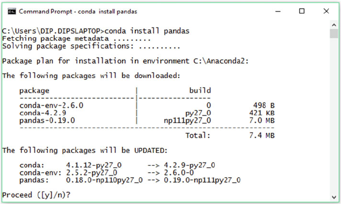
CHAPTER 2 ■ PYTHON REFRESHER

64

The conda package manager is better than pip in several aspects because it provides

a holistic view of which dependencies are going to be upgraded and the specific versions

and other details during installation. Also pip often fails to install some packages in

Windows, but conda has no such issues during installation. Figure

2-4 depicts how to

manage packages using conda .

Now you have a much better idea of how to install external packages and libraries in

Python. This will be useful later when we install some libraries that have been specifically

built for text analytics. Your Python environment should now be set up and ready for

executing code. Before we dive into the basic and advanced concepts in Python, we will

conclude this section with a discussion about virtual environments.

Virtual Environments

A virtual environment , or venv , is a complete isolated Python environment with its own

Python interpreter, libraries, modules, and scripts. This environment is a standalone

environment isolated from other virtual environments and the default system-level

Python environment. Virtual environments are extremely useful when you have multiple

projects or codebases that have dependencies on different versions of the same packages

or libraries. For example, if my project TextApp1 depends on nltk 2.0 and another

project, TextApp2, depends on nltk 3.0 , then it would be impossible to run both projects

on the same system. Hence, the need for virtual environments that provide complete

isolated environments that can be activated and deactivated as needed.

Figure 2-4. Package management using conda

CHAPTER 2 ■ PYTHON REFRESHER

65

To set up a virtual environment, you need to install the virtualenv package as follows:

E:\Apress>pip install virtualenv

Collecting virtualenv

Downloading virtualenv-15.0.2-py2.py3-none-any.whl (1.8MB)

100% |################################| 1.8MB 290kB/s

Installing collected packages: virtualenv

Successfully installed virtualenv-15.0.2

Once installed, you can create a virtual environment as follows, where we create a new

project directory called test_proj and create the virtual environment inside the directory:

E:\Apress>mkdir test_proj && chdir test_proj

E:\Apress\test_proj>virtualenv venv

New python executable in E:\Apress\test_proj\venv\Scripts\python.exe

Installing setuptools, pip, wheel...done.

Once you have installed the virtual environment successfully, you can activate it

using the following command:

E:\Apress\test_proj>venv\Scripts\activate

(venv) E:\Apress\test_proj>python --version

Python 2.7.11 :: Continuum Analytics, Inc.

For other OS platforms, you may need to use the command source venv/bin/

activate to activate the virtual environment.

Once the virtual environment is active, you can see the (venv) notation as shown in

the preceding code output, and any new packages you install will be placed in the venv

folder in complete isolation from the global system Python installation. This difference

is illustrated by depicting different versions for the pandas package in the global system

Python and the virtual environment Python in the following code:

C:\Users\DIP.DIPSLAPTOP>echo 'This is Global System Python'

'This is Global System Python'

C:\Users\DIP.DIPSLAPTOP>pip freeze | grep pandas

pandas==0.18.0

(venv) E:\Apress\test_proj>echo 'This is VirtualEnv Python'

'This is VirtualEnv Python'

(venv) E:\Apress\test_proj>pip install pandas

Collecting pandas

Downloading pandas-0.18.1-cp27-cp27m-win_amd64.whl (6.2MB)

100% |################################| 6.2MB 142kB/s

Installing collected packages: pandas

Successfully installed pandas-0.18.1

(venv) E:\Apress\test_proj>pip freeze | grep pandas

pandas==0.18.1

CHAPTER 2 ■ PYTHON REFRESHER

66

You can see from that code how the pandas package has different versions in the

same machine: 0.18.0 for global Python and 0.18.1 for the virtual environment Python.

Hence, these isolated virtual environments can run seamlessly on the same system.

Once you have finished working in the virtual environment, you can deactivate it

again as follows:

(venv) E:\Apress\test_proj>venv\Scripts\deactivate

E:\Apress\test_proj>

This will bring you back to the system’s default Python interpreter with all its

installed libraries. This gives us a good idea about the utility and advantages of virtual

environments, and once you start working on several projects, you should definitely

consider using it. To find out more about virtual environments, check out

http://docs.

python-guide.org/en/latest/dev/virtualenvs/

, the official documentation for the

virtualenv package.

This brings us to the end of our installation and setup activities, and now we will

be looking into Python concepts, constructs, syntax, and semantics using hands-on

examples.

Python Syntax and Structure

There is a defined hierarchical syntax for Python code that you should remember when

writing code. Any big Python application or system is built using several modules, which

are themselves comprised of Python statements. Each statement is like a command or

direction to the system directing what operations it should perform, and these statements

are comprised of expressions and objects. Everything in Python is an object—including

functions, data structures, types, classes and so on. This hierarchy is visualized in

Figure

2-5 .

Figure 2-5. Python program structure hierarchy

CHAPTER 2 ■ PYTHON REFRESHER

67

The basic statements consist of objects, expressions which usually make use of objects

and process and perform operations on them. Objects can be anything from simple data

types and structures to complex objects, including functions and reserved words that have

their own specific roles. Python has around 37 keywords , or reserved words, which have

their own designated roles and functions. Table

2-1 list each keyword in detail, including

examples that should be useful and handy when you are using them in your code.

Table 2-1. Python Reserved Words

Sl No. Keyword Description Example

1 and The logical AND operator (5==5 and 1==2) == False

2 as Used as a synonym to some

object/reference

with open('file.txt') as f

3 assert Asserts/checks if some

expression is True

assert 1==2, "Not Equal"

4 async Declares a function as

asynchronous (co-routine)

async def get_data():

5 await Used to invoke a co-routine return await get_data()

6 break Breaks out of an executing loop while True:

break

7 class Create a class (OOP) class ClassifyText(object):

8 continue Continue with the next iteration

of the loop

while True:

if a==1: continue

9 def Defines a function def add(a,b):

return a+b

10 del Deletes references del arr

11 elif Else-if conditional if num==1: print '1'

elif num==2: print '2'

12 else Else conditional if num==1: print '1'

else: print 'not 1'

13 except Catch exceptions except ValueError, e: print e

14 exec Dynamic execution of code exec 'print "Hello Python"'

15 False Boolean False False == 0

16 finally Finally execute statements after

try-except

finally: print 'end of

exception'

17 for The for loop for num in arr: print num

18 from

Import specific components

from modules

from nltk.corpus import

brown

19 global Declare variables as global global var

20 if If conditional if num==1: print '1'

(continued)

CHAPTER 2 ■ PYTHON REFRESHER

68

Table 2-1 shows us all of Python’s keywords that are used in statements. However,

there are a few caveats to remember. The async and await keywords are only available

in Python 3.5.x onwards. The exec and print keywords are statements only in Python

2.x—starting from Python 3.x they are functions. The keywords False , True , and nonlocal

were introduced starting with Python 3.x in the keywords list.

Python statements usually direct the interpreter as to what they should do when

executing the statements. A bunch of statements usually forms a logical block of code.

Various constructs including functions and loops and conditionals help in segregating

and executing blocks of code using logic and design based on user decisions. Python also

focuses a lot on readability—hence, indentation is an important part of Python code. By

default, Python does not use punctuation like semicolons to indicate end of statements. It

also uses tabs or whitespaces to indicate and delimit specific blocks of code instead of the

traditional braces or keywords as used in languages like C, C++, Java, and so on. Python

Table 2-1. (continued)

Sl No. Keyword Description Example

21 import Import an existing module import numpy

22 in Check or loop through some

existing object

for num in arr \ if x in y

23 is Used to check for equality type('a') is str

24 lambda Create an anonymous function lambda a: a**a

25 None Represents no value or null num = None

26 nonlocal Modify variable values of an

outer but non global scope in

functions

nonlocal var

27 not The logical NOT operator not 1 == 2

28 or The logical OR operator 1 or 2 == 1

29 pass Used as a placeholder

indicating an empty block

if a == 1: pass

30 print Prints a string or other objects print 'Hello World!'

31 raise Raises an exception raise Exception('overflow')

32 return Returns object(s) from a

function after exiting

return a, b

33 try Tries a code block and goes to

except if exception occurs

try: read_file()

except Exception, e: print e

34 while The while loop while True: print value

35 with With an object in an expression

perform some operation

with open('file.txt') as f:

data = f.read()

36 yield Generator functionality, pause

and return to the caller

def generate_func(arr):

for num in arr: yield num+1

CHAPTER 2 ■ PYTHON REFRESHER

69

accepts both spaces and tabs as indentation, with the usual norm being one tab or four

spaces to indicate each specific block of code. Unindented code will always throw syntax

errors, so anyone writing Python code must be extra careful with code formatting and

indentation.

Python programs are usually structured around the hierarchy mentioned earlier.

Each module is usually a directory with a __init__.py file, which makes the directory

a package, and it may have multiple modules, each of which is an individual Python

( .py ) file . Each module usually has classes and objects like functions that are invoked by

other modules and code. All interconnected modules finally make up a complete Python

program, application, or system. Usually you start any project by writing necessary code

in Python (.py) files and making it modular as it gets bigger by adding more components.

Data Structures and Types

Python has several data types and many are used as data structures for handling data. All

data types are derived from the default object data type in Python. This object data type

is an abstraction used by Python for managing and handling data. Code and data are all

stored and handled by objects and relations among objects. Each object has three things

or properties that distinguish it from other objects:

• Identity : This is unique and never changes once the object is

created and is usually represented by the object’s memory

address.

• Type : This determines the type of object (usually the data type,

which is again a child of the base object type).

• Value : The actual value stored by the object.

Let’s say a variable is holding a string that is one of the data types. To see the three

properties in action, you can use the functions depicted in the following code snippet:

In [46]: new_string = "This is a String" # storing a string

In [47]: id(new_string) # shows the object identifier (address)

Out[47]: 243047144L

In [48]: type(new_string) # shows the object type

Out[48]: str

In [49]: new_string # shows the object value

Out[49]: 'This is a String'

Python has several data types, including several core data types and complex ones

including functions and classes. In this section we will talk about the core data types of

Python, including some that are used extensively as data structures to handle data. These

core data types are as follows:

CHAPTER 2 ■ PYTHON REFRESHER

70

• Numeric

• Strings

• Lists

• Sets

• Dictionaries

• Tuples

• Files

• Miscellaneous

Although that’s not an exhaustive list , more than 90 percent of your time will be

spent writing Python statements that make use of these objects. Let’s discuss each of

them in more detail to understand their properties and behavior better.

Numeric Types

The numeric data type is perhaps the most common and basic data type in Python. All

kinds of applications end up processing and using numbers in some form or the other.

There are mainly three numeric types: integers, floats, and complex numbers. Integers are

numbers that do not have a fractional part or mantissa after the decimal point. Integers

can be represented and operated upon as follows:

In [52]: # representing integers and operations on them

In [53]: num = 123

In [54]: type(num)

Out[54]: int

In [55]: num + 1000 # addition

Out[55]: 1123

In [56]: num * 2 # multiplication

Out[56]: 246

In [59]: num / 2 # integer division

Out[59]: 61

There are also various types of integers, depending on their radix or base. These

include decimal, binary, octal, and hexadecimal integers. Normal nonzero leading

sequences of numbers are decimal integers. Integers that start with a 0 , or often 0o to

prevent making mistakes, are octal integers. Numbers that start with 0x are hexadecimal,

and those starting with 0b are binary integers. You can also make use of the bin() , hex() ,

and oct() functions for converting decimal integers to the respective base form.

CHAPTER 2 ■ PYTHON REFRESHER

71

The following code snippet illustrates the various forms of integers:

In [94]: # decimal

In [95]: 1 + 1

Out[95]: 2

In [96]: # binary

In [97]: bin(2)

Out[97]: '0b10'

In [98]: 0b1 + 0b1

Out[98]: 2

In [99]: bin(0b1 + 0b1)

Out[99]: '0b10'

In [100]: # octal

In [101]: oct(8)

Out[101]: '010'

In [102]: oct(07 + 01)

Out[102]: '010'

In [103]: 0o10

Out[103]: 8

In [104]: # hexadecimal

In [105]: hex(16)

Out[105]: '0x10'

In [106]: 0x10

Out[106]: 16

In [116]: hex(0x16 + 0x5)

Out[116]: '0x1b'

Floating point numbers, or floats, are represented as a sequence of numbers that

include a decimal point and some numbers following it (the mantissa), an exponent part

( e or E followed by a +/- sign followed by digits), or sometimes both of them. Here are

some examples of floating point numbers :

In [126]: 1.5 + 2.6

Out[126]: 4.1

In [127]: 1e2 + 1.5e3 + 0.5

Out[127]: 1600.5

In [128]: 2.5e4

Out[128]: 25000.0

In [129]: 2.5e-2

Out[129]: 0.025

The floating point numbers have a range and precision similar to the double data

type in the C language.

CHAPTER 2 ■ PYTHON REFRESHER

72

Complex numbers have two components, a real and an imaginary component

represented by floating point numbers. The imaginary literal consists of the number

followed by the letter j , and this symbol j at the end of the literal indicates the square root

of –1. The following code snippet shows some representations and operations of complex

numbers:

In [132]: cnum = 5 + 7j

In [133]: type(cnum)

Out[133]: complex

In [134]: cnum.real

Out[134]: 5.0

In [135]: cnum.imag

Out[135]: 7.0

In [136]: cnum + (1 - 0.5j)

Out[136]: (6+6.5j)

S t r i n g s

Strings are sequences or collections of characters used to store and represent textual

data—which will be our data type of choice in most examples in the book. Strings can

be used to store both textual as well as bytes as information. Strings have a wide variety

of methods that can be used for handling and manipulating strings, which we will see in

detail later in this chapter. An important point to remember is that strings are immutable ,

and any operations performed on strings always creates a new string object (remember

the three properties of an object?) rather than just mutating and changing the value of the

existing string object.

The following code snippet shows some string representations and some basic

operations on strings:

In [147]: s1 = 'this is a string'

In [148]: s2 = 'this is "another" string'

In [149]: s3 = 'this is the \'third\' string'

In [150]: s4 = """this is a

...: multiline

...: string"""

In [151]: print s1, s2, s3, s4

this is a string this is "another" string this is the 'third'

string this is a

multiline

string

CHAPTER 2 ■ PYTHON REFRESHER

73

In [152]: print s3 + '\n' + s4

this is the 'third' string

this is a

multiline

string

In [153]: ' '.join([s1, s2])

Out[153]: 'this is a string this is "another" string'

In [154]: s1[::-1] # reverses the string

Out[154]: 'gnirts a si siht'

L i s t s

Lists are collections of arbitrary heterogeneous or homogenous typed objects. Lists also

follow a sequence based on the order in which the objects are present in the list, and

each object has its own index with which it can be accessed. Lists are similar to arrays in

other languages, with the distinction that unlike arrays, which hold homogenous items

of the same type, lists can contain different types of objects. A simple example would be

a list containing numbers, strings, and even sublists. If a list contains objects that are lists

themselves, these are often called nested lists.

The following code snippet shows some examples of lists:

In [161]: l1 = ['eggs', 'flour', 'butter']

In [162]: l2 = list([1, 'drink', 10, 'sandwiches', 0.45e-2])

In [163]: l3 = [1, 2, 3, ['a', 'b', 'c'], ['Hello', 'Python']]

In [164]: print l1, l2, l3

['eggs', 'flour', 'butter'] [1, 'drink', 10, 'sandwiches', 0.0045] [1, 2, 3,

['a', 'b', 'c'], ['Hello', 'Python']]

You can also perform numerous operations on lists, including indexing, slicing,

appending, popping, and many more. Some typical operations on lists are depicted in the

following code snippet:

In [167]: # indexing lists

In [168]: l1

Out[168]: ['eggs', 'flour', 'butter']

In [169]: l1[0]

Out[169]: 'eggs'

In [170]: l1[1]

Out[170]: 'flour'

In [171]: l1[0] +' '+ l1[1]

Out[171]: 'eggs flour'

In [171]: # slicing lists

In [172]: l2[1:3]

Out[172]: ['drink', 10]

CHAPTER 2 ■ PYTHON REFRESHER

74

In [173]: numbers = range(10)

In [174]: numbers

Out[174]: [0, 1, 2, 3, 4, 5, 6, 7, 8, 9]

In [175]: numbers[2:5]

Out[175]: [2, 3, 4]

In [180]: numbers[:]

Out[180]: [0, 1, 2, 3, 4, 5, 6, 7, 8, 9]

In [181]: numbers[::2]

Out[181]: [0, 2, 4, 6, 8]

In [181]: # concatenating and mutating lists

In [182]: numbers * 2

Out[182]: [0, 1, 2, 3, 4, 5, 6, 7, 8, 9, 0, 1, 2, 3, 4, 5, 6, 7, 8, 9]

In [183]: numbers + l2

Out[183]: [0, 1, 2, 3, 4, 5, 6, 7, 8, 9, 1, 'drink', 10, 'sandwiches',

0.0045]

In [184]: # handling nested lists

In [184]: l3

Out[184]: [1, 2, 3, ['a', 'b', 'c'], ['Hello', 'Python']]

In [185]: l3[3]

Out[185]: ['a', 'b', 'c']

In [186]: l3[4]

Out[186]: ['Hello', 'Python']

In [187]: l3.append(' '.join(l3[4])) # append operation

In [188]: l3

Out[188]: [1, 2, 3, ['a', 'b', 'c'], ['Hello', 'Python'], 'Hello Python']

In [189]: l3.pop(3) # pop operation

Out[189]: ['a', 'b', 'c']

In [190]: l3

Out[190]: [1, 2, 3, ['Hello', 'Python'], 'Hello Python']

Sets

Sets are unordered collections of unique and immutable objects. You can use the set()

function or the curly braces {...} to create a new set. Sets are typically used to remove

duplicates from a list, test memberships, and perform mathematical set operations,

including union, intersection, difference, and symmetric difference.

Some set representations and operations are shown in the following code snippet:

In [196]: l1 = [1,1,2,3,5,5,7,9,1]

In [197]: set(l1) # makes the list as a set

Out[197]: {1, 2, 3, 5, 7, 9}

CHAPTER 2 ■ PYTHON REFRESHER

75

In [198]: s1 = set(l1)

# membership testing

In [199]: 1 in s1

Out[199]: True

In [200]: 100 in s1

Out[200]: False

# initialize a second set

In [201]: s2 = {5, 7, 11}

# testing various set operations

In [202]: s1 - s2 # set difference

Out[202]: {1, 2, 3, 9}

In [203]: s1 | s2 # set union

Out[203]: {1, 2, 3, 5, 7, 9, 11}

In [204]: s1 & s2 # set intersection

Out[204]: {5, 7}

In [205]: s1 ^ s2 # elements which do not appear in both sets

Out[205]: {1, 2, 3, 9, 11}

Dictionaries

Dictionaries in Python are key-value mappings that are unordered and mutable. They

are often known as hashmaps , associative arrays , and associative memories . Dictionaries

are indexed using keys , which can be any immutable object type, like numeric types or

strings, or even tuples, which we will see later on. Remember that keys should always

be some immutable data type. Dictionary values can be immutable or mutable objects,

including lists and dictionaries themselves which would lead to nested dictionaries.

Dictionaries have a lot of similarity with JSON objects, if you have worked with them

previously. Dictionaries are often called dicts in Python, and the dict() function is also

used to create new dictionaries.

The following code snippets show some representations and operations on

dictionaries:

In [207]: d1 = {'eggs': 2, 'milk': 3, 'spam': 10, 'ham': 15}

In [208]: d1

Out[208]: {'eggs': 2, 'ham': 15, 'milk': 3, 'spam': 10}

# retrieving items based on key

In [209]: d1.get('eggs')

Out[209]: 2

In [210]: d1['eggs']

Out[210]: 2

CHAPTER 2 ■ PYTHON REFRESHER

76

# get is better than direct indexing since it does not throw errors

In [211]: d1.get('orange')

In [212]: d1['orange']

Traceback (most recent call last):

File "<ipython-input-212-ebecbf415243>", line 1, in <module>

d1['orange']

KeyError: 'orange'

# setting items with a specific key

In [213]: d1['orange'] = 25

In [214]: d1

Out[214]: {'eggs': 2, 'ham': 15, 'milk': 3, 'orange': 25, 'spam': 10}

# viewing keys and values

In [215]: d1.keys()

Out[215]: ['orange', 'eggs', 'ham', 'milk', 'spam']

In [216]: d1.values()

Out[216]: [25, 2, 15, 3, 10]

# create a new dictionary using dict function

In [219]: d2 = dict({'orange': 5, 'melon': 17, 'milk': 10})

In [220]: d2

Out[220]: {'melon': 17, 'milk': 10, 'orange': 5}

# update dictionary d1 based on new key-values in d2

In [221]: d1.update(d2)

In [222]: d1

Out[222]: {'eggs': 2, 'ham': 15, 'melon': 17, 'milk': 10, 'orange': 5,

'spam': 10}

# complex and nested dictionary

In [223]: d3 = {'k1': 5, 'k2': [1,2,3,4,5], 'k3': {'a': 1, 'b': 2, 'c':

[1,2,3]}}

In [225]: d3

Out[225]: {'k1': 5, 'k2': [1, 2, 3, 4, 5], 'k3': {'a': 1, 'b': 2, 'c':

[1, 2, 3]}}

In [226]: d3.get('k3')

Out[226]: {'a': 1, 'b': 2, 'c': [1, 2, 3]}

In [227]: d3.get('k3').get('c')

Out[227]: [1, 2, 3]

Tuples

Tuples are also sequences like lists, but they are immutable. Typically, tuples are used

to represent fixed collections of objects or values. Tuples are created using a comma-

separated sequence of values enclosed by parentheses, and optionally the tuple()

function can also be used.

CHAPTER 2 ■ PYTHON REFRESHER

77

The following code snippet shows some representations and operations on tuples:

# creating a tuple with a single element

In [234]: single_tuple = (1,)

In [235]: single_tuple

Out[235]: (1,)

# original address of the tuple

In [239]: id(single_tuple)

Out[239]: 176216328L

# modifying contents of the tuple but its location changes (new tuple is

created)

In [240]: single_tuple = single_tuple + (2, 3, 4, 5)

In [241]: single_tuple

Out[241]: (1, 2, 3, 4, 5)

In [242]: id(single_tuple) # different address indicating new tuple with

same name

Out[242]: 201211312L

# tuples are immutable hence assignment is not supported like lists

In [243]: single_tuple[3] = 100

Traceback (most recent call last):

File "<ipython-input-247-37d1946d4128>", line 1, in <module>

single_tuple[3] = 100

TypeError: 'tuple' object does not support item assignment

# accessing and unpacking tuples

In [243]: tup = (['this', 'is', 'list', '1'], ['this', 'is', 'list', '2'])

In [244]: tup[0]

Out[244]: ['this', 'is', 'list', '1']

In [245]: l1, l2 = tup

In [246]: print l1, l2

['this', 'is', 'list', '1'] ['this', 'is', 'list', '2']

Files

Files are special types of objects in Python that are used mainly for interfacing with

external objects in the filesystem, including text, binary, audio, and video files, plus

documents, images, and many more. Some might disagree about it being a data type in

Python, but it actually is a special data type, and the name of the type, file, suits its role

perfectly for handling all types of external files. You usually use the open() function to

open a file, and there are various modes like read and write that are specified using a

processing mode character in the function.

Some examples of file handling are show in the following code snippet:

CHAPTER 2 ■ PYTHON REFRESHER

78

In [253]: f = open('text_file.txt', 'w') # open in write mode

In [254]: f.write("This is some text\n") # write some text

In [255]: f.write("Hello world!")

In [256]: f.close() # closes the file

# lists files in current directory

In [260]: import os

In [262]: os.listdir(os.getcwd())

Out[262]: ['text_file.txt']

In [263]: f = open('text_file.txt', 'r') # opens file in read mode

In [264]: data = f.readlines() # reads in all lines from file

In [265]: print data # prints the text data

['This is some text\n', 'Hello world!']

Miscellaneous

Besides the already mentioned data types and structures, there are several other Python

data types:

• The None type indicates no value/no data or null object.

• Boolean types include True and False.

• Decimal and Fraction types handle numbers in a better way.

This completes the list for Python’s core data types and data structures that you will

be using most of the time in your code and implementations. We will now discuss some

constructs typically used for controlling the flow of code.

Controlling Code Flow

Flow of code is extremely important. A lot of it is based on business logic and rules. It also

depends on the type of implementation decisions developers take when building systems

and applications. Python provides several control flow tools and utilities that can be used

to control the flow of your code. Here are the most popular ones:

• if-elif-else conditionals

• for loop

• while loop

• break, continue, and else in loops

• try-except

These constructs will help you understand several concepts including conditional

code flow, looping, and handling exceptions.

CHAPTER 2 ■ PYTHON REFRESHER

79

Conditional Constructs

The concept of conditional code flow involves executing different blocks of code

conditionally based on some user-defined logic implemented in the code itself. It is

extremely useful when you do not want to execute a block of statements sequentially

one after the other but execute a part of them based on fulfilling or not fulfilling certain

conditions. The if-elif-else statements help in achieving this. The general syntax for it is as

follows:

if <conditional check 1 is True>: # the if conditional (mandatory)

<code block 1> # executed only when check 1 evaluates to True

...

elif <conditional check 2 is True>: # the elif conditional (optional)

<code block 2> # executed only when check 1 is False and 2 is True

...

else: # the else conditional (optional)

<code block 3> # executed only when check 1 and 2 are False

...

An important point to remember from the preceding syntax is that the corresponding

code blocks only execute based on satisfying the necessary conditions. Also, only the if

statement is mandatory, and the elif and else statements do not need to be mentioned

unless there is a need based on conditional logic.

The following examples depict conditional code flow:

In [270]: var = 'spam'

In [271]: if var == 'spam':

...: print 'Spam'

...:

Spam

In [272]: var = 'ham'

In [273]: if var == 'spam':

...: print 'Spam'

...: elif var == 'ham':

...: print 'Ham'

...:

Ham

CHAPTER 2 ■ PYTHON REFRESHER

80

In [274]: var = 'foo'

In [275]: if var == 'spam':

...: print 'Spam'

...: elif var == 'ham':

...: print 'Ham'

...: else:

...: print 'Neither Spam or Ham'

...:

Neither Spam or Ham

Looping Constructs

There are two main types of loops in Python: for and while loops. These looping

constructs are used to execute blocks of code repeatedly until some condition is satisfied

or the loop exits based on some other statements or conditionals.

The for statement is generally used to loop through items in sequence and usually

loops through one or many iterables sequentially, executing the same block of code in

each turn. The while statement is used more as a conditional general loop, which stops

the loop once some condition is satisfied or runs the loop till some condition is satisfied.

Interestingly, there is an optional else statement at the end of the loops that is executed

only if the loop exits normally without any break statements. The break statement is often

used with a conditional to stop executing all statements in the loop immediately and exit the

closest enclosing loop. The continue statement stops executing all statements below it in

the loop and brings back control to the beginning of the loop for the next iteration. The pass

statement is just used as an empty placeholder—it does not do anything and is often used to

indicate an empty code block . These statements constitute the core looping constructs.

The following snippets show the typical syntax normally used when constructing for

and while loops:

# the for loop

for item in iterable: # loop through each item in the iterable

<code block> # Code block executed repeatedly

else: # Optional else

<code block> # code block executes only if loop exits normally

without 'break'

# the while loop

while <condition>: # loop till condition is satisfied

<code block> # Code block executed repeatedly

else: # Optional else

<code block> # code block executes only if loop exits normally

without 'break'

The following examples show how loops work along with the other looping

constructs including pass , break , and continue :

# illustrating for loops

In [280]: numbers = range(0,5)

In [281]: for number in numbers:

...: print number

...:

CHAPTER 2 ■ PYTHON REFRESHER

81

0

1

2

3

4

In [282]: sum = 0

In [283]: for number in numbers:

...: sum += number

...:

In [284]: print sum

10

# role of the trailing else and break constructs

In [285]: for number in numbers:

...: print number

...: else:

...: print 'loop exited normally'

...:

0

1

2

3

4

loop exited normally

In [286]: for number in numbers:

...: if number < 3:

...: print number

...: else:

...: break

...: else:

...: print 'loop exited normally'

...:

0

1

2

# illustrating while loops

In [290]: number = 5

In [291]: while number > 0:

...: print number

...: number -= 1 # important! else loop will keep running

...:

5

4

3

2

1

CHAPTER 2 ■ PYTHON REFRESHER

82

# role of continue construct

In [295]: number = 10

In [296]: while number > 0:

...: if number % 2 != 0:

...: number -=1 # decrement but do not print odd numbers

...: continue # go back to beginning of loop for next

iteration

...: print number # print even numbers and decrement count

...: number -= 1

...:

10

8

6

4

2

# role of the pass construct

In [297]: number = 10

In [298]: while number > 0:

...: if number % 2 != 0:

...: pass # don't print odds

...: else:

...: print number

...: number -= 1

...:

10

8

6

4

2

Handling Exceptions

Exceptions are specific events that are either triggered when some unnatural error

occurs or manually. They are used extensively for error handling, event notifications, and

controlling code flow. Using constructs like try-except-finally , you can make Python

raise exceptions when executing code whenever any error occurs at runtime. This would

also enable you to catch these exceptions and handle them as needed or ignore them

altogether. In Python versions prior to 2.5.x, there were generally two versions of exception

handling using the try construct. One would be try-finally , and the other would involve

try-except and optionally an else clause at the end for catching exceptions. Now we have

a construct that includes them all, the try-except-else-finally construct, which can be

used for exception handling. The syntax is depicted as follows:

try: # The try statement

<main code block> # Checks for errors in this block

except <ExceptionType1>: # Catch different exceptions

CHAPTER 2 ■ PYTHON REFRESHER

83

except <ExceptionType2>:

...

else: # Optional else statement

<optional else block> # Executes only if there were no exceptions

finally: # The finally statement

<finally block> # Always executes in the end

The flow of code in the preceding code snippet starts from the try statement and

the main code block in it, which is executed first and checked for any exceptions. If

any exceptions occur, they are matched based on the exception types as depicted in

the preceding snippet. Assuming ExceptionType1 matches, the exception handler for

ExceptionType1 is executed, which is exception handler 1 . In case no exceptions were

raised, only then the optional else block is executed. The finally block is always

executed irrespective of any exceptions being raised or not.

The following examples depict the use of the try-except-else-finally construct:

In [311]: shopping_list = ['eggs', 'ham', 'bacon']

# trying to access a non-existent item in the list

In [312]: try:

...: print shopping_list[3]

...: except IndexError as e:

...: print 'Exception: '+str(e)+' has occurred'

...: else:

...: print 'No exceptions occurred'

...: finally:

...: print 'I will always execute no matter what!'

...:

Exception: list index out of range has occurred

I will always execute no matter what!

# smooth code execution without any errors

In [313]: try:

...: print shopping_list[2]

...: except IndexError as e:

...: print 'Exception: '+str(e)+' has occurred'

...: else:

...: print 'No exceptions occurred'

...: finally:

...: print 'I will always execute no matter what!'

...:

bacon

No exceptions occurred

I will always execute no matter what!

This brings us to the end of our discussion on the core constructs for controlling flow

of code in Python. The next section covers some core concepts and constructs that are

parts of the functional programming paradigm in Python.

CHAPTER 2 ■ PYTHON REFRESHER

84

Functional Programming

The functional programming paradigm is a style of programming with origins in lambda

calculus. It treats any form of computation purely on the basis of executing and evaluating

functions. Python is not a pure functional programming language but does have several

constructs that can be used for functional programming. In this section we will talk

about several of these constructs, including functions and some advanced concepts like

generators, iterators, and comprehensions. We will also look at modules like itertools

and functools that contain implementation of functional tools based on concepts from

Haskell and Standard ML.

Functions

A function can be defined as a block of code that is executed only on request by invoking

it. Functions consist of a function definition that has the function signature (function

name, parameters) and a group of statements inside the function that are executed when

the function is called. The Python standard library provides a huge suite of functions to

choose from to perform different types of operations. Besides this, users can define their

own functions using the def keyword.

Functions usually return some value always, and even when they do not return a

value, by default they return the None type. One important thing to remember is that often

you may see methods and functions being used interchangeably, but the distinction

between functions and methods is that methods are functions that are defined within

class statements. Functions are also objects, since each and every type and construct in

Python is derived from the base object type. This opens up a whole new dimension where

you can even pass functions as parameters or arguments to other functions. Moreover,

functions can be bound to variables and even returned as results from other functions.

Hence functions are often known as first-class objects in Python.

The following code snippet shows the basic structure of a function definition in

Python:

def function(params): # params are the input parameters

<code block> # code block consists of a group of statements

return value(s) # optional return statement

The params indicate the list of input parameters, which are not mandatory, and in

many functions there are actually no input parameters. You can even pass functions

themselves as parameters. Some logic executes in the code block, which may or may not

modify the input parameters, and finally you may return some output values or not return

anything entirely.

The following code snippets demonstrate some basic examples of functions with

fixed arguments, variable arguments, and built-in functions:

# function with single argument

In [319]: def square(number):

...: return number*number

...:

CHAPTER 2 ■ PYTHON REFRESHER

85

In [320]: square(5)

Out[320]: 25

# built-in function from the numpy library

In [321]: import numpy as np

In [322]: np.square(5)

Out[322]: 25

# a more complex function with variable number of arguments

In [323]: def squares(*args):

...: squared_args = []

...: for item in args:

...: squared_args.append(item*item)

...: return squared_args

...:

In [324]: squares(1,2,3,4,5)

Out[324]: [1, 4, 9, 16, 25]

The preceding example shows how to introduce variable number of arguments in a

function dynamically. You can also introduce keyword arguments, where each argument

has its own variable name and value, as illustrated in the following code snippet:

# assign specific keyword based arguments dynamically

In [325]: def person_details(**kwargs):

...: for key, value in kwargs.items():

...: print key, '->', value

...:

In [326]: person_details(name='James Bond', alias='007', job='Secret Service

Agent')

alias -> 007

job -> Secret Service Agent

name -> James Bond

Recursive Functions

Recursive functions use the concept of recursion , wherein the function calls itself inside

its code block. Care should be taken to make sure there is a stopping condition that

ultimately terminates the recursive calls—otherwise the function will run into an endless

loop of execution where it goes on calling itself. Recursion makes use of the call stack at

each recursive call, hence they are often not very efficient compared to regular functions;

nevertheless, they are extremely powerful.

The following example depicts our squares function using recursion:

# using recursion to square numbers

In [331]: def recursive_squares(numbers):

...: if not numbers:

...: return []

CHAPTER 2 ■ PYTHON REFRESHER

86

...: else:

...: return [numbers[0]*numbers[0]] + recursive_

squares(numbers[1:])

...:

In [332]: recursive_squares([1, 2, 3, 4, 5])

Out[332]: [1, 4, 9, 16, 25]

Anonymous Functions

Anonymous functions are functions that do not have any name and usually consist of

a one-line expression that denotes a function using the lambda construct. The lambda

keyword is used to define inline function objects that can be used just like regular

functions, with a few differences. The general syntax for a lambda function is shown in the

following code snippet:

lambda arg, arg2,... arg_n : <inline expression using args>

This expression can actually be even assigned to variables and then executed as a

normal function call similar to functions created with def . However, lambda functions are

expressions and never statements like the code block inside a def , and so it is extremely

difficult to put complex logic inside a lambda function because it is always a single-lined

inline expression. However, lambda functions are very powerful and are even used inside

lists, functions, and function arguments. Besides lambda functions, Python also provides

functions like map() , reduce() , and filter() , which make extensive use of lambda

functions and apply them to iterables usually to transform, reduce, or filter respectively.

The following code snippet depicts some examples of lambda functions used with the

constructs we just talked about:

# simple lambda function to square a number

In [340]: lambda_square = lambda n: n*n

In [341]: lambda_square(5)

Out[341]: 25

# map function to square numbers using lambda

In [342]: map(lambda_square, [1, 2, 3, 4, 5])

Out[342]: [1, 4, 9, 16, 25]

# lambda function to find even numbers used for filtering

In [343]: lambda_evens = lambda n: n%2 == 0

In [344]: filter(lambda_evens, [1, 2, 3, 4, 5, 6, 7, 8, 9, 10])

Out[344]: [2, 4, 6, 8, 10]

# lambda function to add numbers used for adding numbers in reduce function

In [345]: lambda_sum = lambda x, y: x + y

In [346]: reduce(lambda_sum, [1, 2, 3, 4, 5])

Out[346]: 15

CHAPTER 2 ■ PYTHON REFRESHER

87

# lambda function to make a sentence from word tokens with reduce function

In [347]: lambda_sentence_maker = lambda word1, word2: ' '.join([word1,

word2])

In [348]: reduce(lambda_sentence_maker, ['I', 'am', 'making', 'a',

'sentence', 'from', 'words!'])

Out[348]: 'I am making a sentence from words!'

The preceding examples should give you a pretty good idea about how lambda

functions work and how powerful they are. Using a one-line construct you can create

free-flowing sentences from word tokens and calculate a sum of numbers in a list! The

possibilities of using lambda functions are endless, and you can use them to solve even

the most complex of problems.

I t e r a t o r s

Iterators are constructs used to iterate through iterables. Iterables are objects that are

basically sequences of other objects and data. A good example would be a for loop, which is

actually an iterable that iterates through a list or sequence. Iterators are objects or constructs

that can be used to iterate through iterables using the next() function, which returns the next

item from the iterable at each call. Once it has iterated through the entire iterable, it returns

a StopIteration exception. We have seen how a for loop works in general, however behind

the abstraction, the for loop actually calls the iter() function on the iterable to create an

iterator object and then traverses through it using the next() function.

The following example illustrates how iterators work:

# typical for loop

In [350]: numbers = range(6)

In [351]: for number in numbers:

...: print number

0

1

2

3

4

5

# illustrating how iterators work behind the scenes

In [352]: iterator_obj = iter(numbers)

In [353]: while True:

...: try:

...: print iterator_obj.next()

...: except StopIteration:

...: print 'Reached end of sequence'

...: break

0

1

2

CHAPTER 2 ■ PYTHON REFRESHER

88

3

4

5

Reached end of sequence

# calling next now would throw the StopIteration exception as expected

In [354]: iterator_obj.next()

Traceback (most recent call last):

File "<ipython-input-354-491178c4f97a>", line 1, in <module>

iterator_obj.next()

StopIteration

Comprehensions

Comprehensions are interesting constructs that are similar to for loops but more

efficient. They fall rightly into the functional programming paradigm following the set

builder notation. Originally, the idea for list comprehensions came from Haskell, and

after a series of lengthy discussions comprehensions were finally added and have been

one of the most used constructs ever since. There are various types of comprehensions

that can be applied on existing data types, including list, set, and dict comprehensions.

The following code snippet shows the syntax of comprehensions using the very common

list comprehensions and for loops, a core component in comprehensions:

# typical comprehension syntax

[ expression for item in iterable ]

# equivalent for loop statement

for item in iterable:

expression

# complex and nested iterations

[ expression for item1 in iterable1 if condition1

for item2 in iterable2 if condition2 ...

for itemN in iterableN if conditionN ]

# equivalent for loop statement

for item1 in iterable1:

if condition1:

for item2 in iterable2:

if condition2:

...

for itemN in iterableN:

if conditionN:

expression

CHAPTER 2 ■ PYTHON REFRESHER

89

This gives us an idea of how similar comprehensions are to looping constructs. The

benefit we get is that they are more efficient and perform better than loops. Some caveats

include that you cannot use assignment statements in comprehensions because, if you

remember the syntax from earlier, they support only expressions and not statements. The

same syntax is used by set and dictionary comprehensions too.

The following examples illustrate the use of different comprehensions :

In [355]: numbers = range(6)

In [356]: numbers

Out[356]: [0, 1, 2, 3, 4, 5]

# simple list comprehension to compute squares

In [357]: [num*num for num in numbers]

Out[357]: [0, 1, 4, 9, 16, 25]

# list comprehension to check if number is divisible by 2

In [358]: [num%2 for num in numbers]

Out[358]: [0, 1, 0, 1, 0, 1]

# set comprehension returns distinct values of the above operation

In [359]: set(num%2 for num in numbers)

Out[359]: {0, 1}

# dictionary comprehension where key:value is number: square(number)

In [361]: {num: num*num for num in numbers}

Out[361]: {0: 0, 1: 1, 2: 4, 3: 9, 4: 16, 5: 25}

# a more complex comprehension showcasing above operations in a single

comprehension

In [362]: [{'number': num,

'square': num*num,

'type': 'even' if num%2 == 0 else 'odd'} for num in numbers]

Out[362]:

[{'number': 0, 'square': 0, 'type': 'even'},

{'number': 1, 'square': 1, 'type': 'odd'},

{'number': 2, 'square': 4, 'type': 'even'},

{'number': 3, 'square': 9, 'type': 'odd'},

{'number': 4, 'square': 16, 'type': 'even'},

{'number': 5, 'square': 25, 'type': 'odd'}]

# nested list comprehension - flattening a list of lists

In [364]: list_of_lists = [[1, 2, 3, 4], [5, 6, 7, 8], [9, 10, 11, 12]]

In [365]: list_of_lists

Out[365]: [[1, 2, 3, 4], [5, 6, 7, 8], [9, 10, 11, 12]]

In [367]: [item for each_list in list_of_lists for item in each_list]

Out[367]: [1, 2, 3, 4, 5, 6, 7, 8, 9, 10, 11, 12]

CHAPTER 2 ■ PYTHON REFRESHER

90

Generators

Generators are powerful, memory-efficient constructs for creating and consuming

iterators. They exist in two variants: functions and expressions. Generators work on a

concept known as lazy evaluation —hence, they are more memory efficient and perform

better in most cases because they do not require the entire object to be evaluated

and loaded in one go, as in list comprehensions. However, the caveat is that because

generators yield one item at a time in an ad hoc fashion, there is a chance that they may

perform worse in terms of execution time compared to list comprehensions, unless you

are dealing with large objects with many elements.

Generator functions are implemented as regular functions using the def statement.

However, they use the concept of lazy evaluation and return one object at a time using

the yield statement. Unlike regular functions that have a return statement, which once

executed ends the execution of the code block inside the function, generators use the

yield statement, which suspends and resumes execution and the state after generating

and returning each value or object. To be more precise, generator functions yield values

at each step rather than returning them. This ensures that the current state including

information about the local code block scope it retained and enables the generator to

resume from where it left off.

The following snippet shows some examples for generator functions:

In [369]: numbers = [1, 2, 3, 4, 5]

In [370]: def generate_squares(numbers):

...: for number in numbers:

...: yield number*number

In [371]: gen_obj = generate_squares(numbers)

In [372]: gen_obj

Out[372]: <generator object generate_squares at 0x000000000F2FC2D0>

In [373]: for item in gen_obj:

...: print item

...:

1

4

9

16

25

The advantages of these generators are both memory efficiency and execution time,

especially when iterables and objects are large in size and occupy substantial memory.

You also do not need to load whole objects into the main memory for performing various

operations on them. They often work very well on streaming data where you cannot keep

all the data in memory at all times. The same applies for generator expressions, which are

very similar to comprehensions except they are enclosed in parentheses.

CHAPTER 2 ■ PYTHON REFRESHER

91

The following example illustrates:

In [381]: csv_string = 'The,fox,jumps,over,the,dog'

# making a sentence using list comprehension

In [382]: list_cmp_obj = [item for item in csv_string.split(',')]

In [383]: list_cmp_obj

Out[383]: ['The', 'fox', 'jumps', 'over', 'the', 'dog']

In [384]: ' '.join(list_cmp_obj)

Out[384]: 'The fox jumps over the dog'

# making a sentence using generator expression

In [385]: gen_obj = (item for item in csv_string.split(','))

In [386]: gen_obj

Out[386]: <generator object <genexpr> at 0x000000000F2FC3F0>

In [387]: ' '.join(gen_obj)

Out[387]: 'The fox jumps over the dog'

Both generator functions and expressions create generator objects that use the same

construct as iterators and starts, stops, and resumes the function or loop at each stage,

and once it is completed it raises the StopIteration exception.

The itertools and functools Modules

Various modules which are available in the Python standard library. Some of the popular

ones include collections , itertools , and functools , which have various constructs and

functions that can be used to boost productivity and reduce time spent writing extra code

to solve problems. The itertools module is a complete module dedicated to building and

operating on iterators. It has various functions that support different operations including

slicing, chaining, grouping, and splitting iterators. The most comprehensive source of

information for itertools is available in the official Python documentation at

https://

docs.python.org/2/library/itertools.html

. The documentation lists each function

and its role with examples. The functools module provides with functions, which enable

concepts from functional programming, including wrappers and partials. These functions

usually act on other functions, which it takes as input parameters and often returns a

function as the result itself. The official documentation at

https://docs.python.org/2/

library/functools.html

provides extensive information on each function.

Classes

Python classes are constructs that enable us to write code following the OOP paradigm.

Concepts like objects, encapsulation, methods, inheritance, and polymorphism are heavily

used in this paradigm. If you have worked on any OOP language before, like C++ or Java,

chances are you will find using Python classes relatively similar to using classes in other

languages. Discussing each concept would be beyond the scope of this book, but I will briefly

cover the basic concepts of classes and touch up on different types of objects and inheritance.

CHAPTER 2 ■ PYTHON REFRESHER

92

Classes are basically a software model or abstraction of real-world entities that

are objects. This abstraction leads to classes being called as a user-defined type, and

once you define a class, you can instantiate and create instances or objects of that class.

Each object has its own instance variables and methods that define the properties and

behavior of that object. All classes inherit from the base object type, and you can create

your own classes and inherit further classes from these user-defined classes. Classes are

also ultimately objects on their own and can be bound to variables and other constructs.

The following snippet gives the basic syntax for a class:

class ClassName(BaseClass):

class_variable # shared by all instances\objects

def __init__(self, ...): # the constructor

# instance variables unique to each instance\object

self.instance_variables = ...

def __str__(self): # string representation of the instance\object

return repr(self)

def methods(self, ...): # instance methods

The preceding snippet tells us that the class named ClassName inherits from

its parent class BaseClass . There can be more than one parent or base class in the

parameters separated by commas. The __init__() method acts as a constructor

that instantiates and creates an object of the class using the call ClassName(...) ,

which automatically invokes the __init__() method—which may optionally take

parameters based on its definition. The __str__() method is optional. It prints the string

representation of the object. You can modify the default method with your own definition,

and it is often used to print the current state of the object variables. The class_variable

indicates class variables that are defined in the block just enclosing the class definition,

and these class variables are shared by all objects or instances of the class. The instance_

variables are variables that are specific to each object or instance. The methods denote

instance methods that define specific behavior of the objects. The self parameter is

usually used as the first parameter in methods, which is more of a convention that refers

to the instance or object of ClassName on which you call the method.

The following example depicts a simple class and how it works:

# class definition

In [401]: class Animal(object):

...: species = 'Animal'

...:

...: def __init__(self, name):

...: self.name = name

...: self.attributes = []

...:

...: def add_attributes(self, attributes):

...: self.attributes.extend(attributes) \

CHAPTER 2 ■ PYTHON REFRESHER

93

...: if type(attributes) == list \

...: else self.attributes.append(attributes)

...:

...: def __str__(self):

...: return self.name+" is of type "+self.species+" and has

attributes:"+str(self.attributes)

...:

# instantiating the class

In [402]: a1 = Animal('Rover')

# invoking instance method

In [403]: a1.add_attributes(['runs', 'eats', 'dog'])

# user defined string representation of the Animal class

In [404]: str(a1)

Out[404]: "Rover is of type Animal and has attributes:['runs', 'eats',

'dog']"

This gives us an idea of how classes work. But what if we want to target specific

animals like dogs and foxes ? We can apply the concept of inheritance and use the super()

method to access the constructor of the base Animal class in each definition. The

following examples illustrate the concept of inheritance:

# deriving class Dog from base class Animal

In [413]: class Dog(Animal):

...: species = 'Dog'

...:

...: def __init__(self, *args):

...: super(Dog, self).__init__(*args)

# deriving class Fox from base class Animal

In [414]: class Fox(Animal):

...: species = 'Fox'

...:

...: def __init__(self, *args):

...: super(Fox, self).__init__(*args)

# creating instance of class Dog

In [415]: d1 = Dog('Rover')

In [416]: d1.add_attributes(['lazy', 'beige', 'sleeps', 'eats'])

In [417]: str(d1)

Out[417]: "Rover is of type Dog and has attributes:['lazy', 'beige',

'sleeps', 'eats']"

# creating instance of class Fox

In [418]: f1 = Fox('Silver')

In [419]: f1.add_attributes(['quick', 'brown', 'jumps', 'runs'])

In [420]: str(f1)

Out[420]: "Silver is of type Fox and has attributes:['quick', 'brown',

'jumps', 'runs']"

CHAPTER 2 ■ PYTHON REFRESHER

94

Working with Text

We have seen most of the constructs, data types, structures, concepts, and programming

paradigms associated with Python in the previous sections. This section briefly covers

specific data types tailored to handle text data and shows how these data types and their

associated utilities will be useful for us in the future chapters. The main data types used to

handle text data in Python are strings, which can be normal strings, bytes storing binary

information, or Unicode. By default, all strings are Unicode in Python 3.x , but they are not

so in Python 2.x, and this is something you should definitely keep in mind when dealing

with text in different Python distributions. Strings are a sequence of characters in Python

similar to arrays and code with a set of attributes and methods that can be leveraged to

manipulate and operate on text data easily, which makes Python the language of choice

for text analytics in many scenarios. We will discuss various types of strings with several

examples in the next section.

String Literals

There are various types of strings, as mentioned earlier, and you saw a few examples in

one of the previous sections regarding data types. The following BNF (Backus-Naur Form )

gives us the general lexical definitions for producing strings as seen in the official Python

docs:

stringliteral ::= [stringprefix](shortstring | longstring)

stringprefix ::= "r" | "u" | "ur" | "R" | "U" | "UR" | "Ur" | "uR"

| "b" | "B" | "br" | "Br" | "bR" | "BR"

shortstring ::= "'" shortstringitem* "'" | '"' shortstringitem* '"'

longstring ::= "'''" longstringitem* "'''" | '"""' longstringitem*

'"""'

shortstringitem ::= shortstringchar | escapeseq

longstringitem ::= longstringchar | escapeseq

shortstringchar ::= <any source character except "\" or newline or the

quote>

longstringchar ::= <any source character except "\">

escapeseq ::= "\" <any ASCII character>

The preceding rules tell us that different types of string prefixes exist that can be used

with different string types to produce string literals. In simple terms, the following types of

string literals are used the most:

• Short strings : These strings are usually enclosed with single ( ' ) or

double quotes ( " ) around the characters. Some examples would

be, 'Hello' and "Hello" .

• Long strings : These strings are usually enclosed with three

single ( ''' ) or double quotes ( """ ) around the characters. Some

examples would be, """Hello, I’m a long string""" or

'''Hello I\’m a long string ''' . Note the ( \’ ), indicates an

escape sequence discussed in the next bullet.

CHAPTER 2 ■ PYTHON REFRESHER

95

• Escape sequences in strings : These strings often have escape

sequences embedded in them, where the rule for escape

sequences starts with a backslash ( \ ) followed by any ASCII

character. Hence, they perform backspace interpolation. Popular

escape sequences include ( \n ), indicating a new line character,

and ( \t ), indicating a tab.

• Bytes : These are used to represent bytestrings, which create

objects of the bytes data type. These strings can be created as

bytes('...') or using the b'...' notation. Examples would be

bytes('hello') and b'hello' .

• Raw strings : These strings were originally created specifically for

regular expressions (regex) and creating regex patterns. These

strings can be created using the r'...' notation and keep the

string in its raw or native form. Hence, it does not perform any

backspace interpolation and turns off the escape sequences. An

example would be r'Hello' .

• Unicode : These strings support Unicode characters in text and

are usually non-ASCII character sequences. These strings are

denoted with the u'...' notation. Besides the string notation,

there are several specific ways to represent special Unicode

characters in the string. The usual include the hex byte value

escape sequence of the format '\xVV' . Besides this, we also

have Unicode escape sequences of the form '\uVVVV' and '\

uVVVVVVVV', where the first form uses 4 hex-digits for encoding

a 16-bit character, and the second uses 8 hex digits for encoding

a 32-bit character. Some examples would be u 'H\xe8llo' and u

'H\u00e8llo' which represents the string 'Hèllo' .

The following code snippet depicts these different types of string literals and their

output:

# simple string

In [422]: simple_string = 'hello' + " I'm a simple string"

In [423]: print simple_string

hello I'm a simple string

# multi-line string, note the \n (newline) escape character automatically

created

In [424]: multi_line_string = """Hello I'm

...: a multi-line

...: string!"""

In [425]: multi_line_string

Out[425]: "Hello I'm\na multi-line\nstring!"

In [426]: print multi_line_string

Hello I'm

a multi-line

string!

CHAPTER 2 ■ PYTHON REFRESHER

96

# Normal string with escape sequences leading to a wrong file path!

In [427]: escaped_string = "C:\the_folder\new_dir\file.txt"

In [428]: print escaped_string # will cause errors if we try to open a file

here

C: he_folder

ew_dirile.txt

# raw string keeping the backslashes in its normal form

In [429]: raw_string = r'C:\the_folder\new_dir\file.txt'

In [430]: print raw_string

C:\the_folder\new_dir\file. txt

# unicode string literals

In [431]: string_with_unicode = u'H\u00e8llo!'

...: print string_with_unicode

Hèllo!

String Operations and Methods

Strings are iterable sequences, which means a lot of operations can be performed on

them, useful especially when processing and parsing textual data into easy-to-consume

formats. Several operations can be performed on strings. I have categorized them into the

following segments:

• Basic operations

• Indexing and slicing

• Methods

• Formatting

• Regular expressions

These would cover the most frequently used techniques for working with strings and

form the base of what we would need to get started in the next chapter (where we look at

understanding and processing textual data based on concepts we learned in the first two

chapters).

Basic Operations

You can perform several basic operations on strings, including concatenation and

checking for substrings, characters, and lengths. The following code snippet illustrates

these operations with some examples:

# Different ways of String concatenation

In [436]: 'Hello' + ' and welcome ' + 'to Python!'

Out[436]: 'Hello and welcome to Python!'

In [437]: 'Hello' ' and welcome ' 'to Python!'

Out[437]: 'Hello and welcome to Python!'

CHAPTER 2 ■ PYTHON REFRESHER

97

# concatenation of variables and literals

In [438]: s1 = 'Python!'

In [439]: 'Hello ' + s1

Out[439]: 'Hello Python!'

# we cannot concatenate a variable and a literal using this method

In [440]: 'Hello ' s1

File "<ipython-input-440-2f801ddf3480>", line 1

'Hello ' s1

^

SyntaxError: invalid syntax

# some more ways of concatenating strings

In [442]: s2 = '--Python--'

In [443]: s2 * 5

Out[443]: '--Python----Python----Python----Python----Python--'

In [444]: s1 + s2

Out[444]: 'Python!--Python--'

In [445]: (s1 + s2)*3

Out[445]: 'Python!--Python--Python!--Python--Python!--Python--'

# concatenating several strings together in parentheses

In [446]: s3 = ('This '

...: 'is another way '

...: 'to concatenate '

...: 'several strings!')

In [447]: s3

Out[447]: 'This is another way to concatenate several strings!'

# checking for substrings in a string

In [448]: 'way' in s3

Out[448]: True

In [449]: 'python' in s3

Out[449]: False

# computing total length of the string

In [450]: len(s3)

Out[450]: 51

Indexing and Slicing

As mentioned, strings are iterables—ordered sequences of characters. Hence they can

be indexed, sliced, and iterated through similarly to other iterables such as lists. Each

character has a specific position in the string, called its index . Using indexes, we can

access specific parts of the string. Accessing a single character using a specific position

or index in the string is called indexing , and accessing a part of a string, for example,

a substring using a start and end index, is called slicing . Python supports two types of

CHAPTER 2 ■ PYTHON REFRESHER

98

indexes. One starts from 0 and increases by 1 each time per character till the end of the

string. The other starts from –1 at the end of the string and decreases by 1 each time for

each character till the beginning of the string . Figure

2-6 shows the two types of indexes

for the string 'PYTHON' .

To access any particular character in the string, you need to use the corresponding

index, and slices can be extracted using the syntax var[start:stop] , which extracts all

characters in the string var from index start till index stop excluding the character at the

stop index.

The following examples shows how to index, slice, and iterate through strings:

# creating a string

In [460]: s = 'PYTHON'

# depicting string indexes

In [461]: for index, character in enumerate(s):

...: print 'Character', character+':', 'has index:', index

Character P: has index: 0

Character Y: has index: 1

Character T: has index: 2

Character H: has index: 3

Character O: has index: 4

Character N: has index: 5

# string indexing

In [462]: s[0], s[1], s[2], s[3], s[4], s[5]

Out[462]: ('P', 'Y', 'T', 'H', 'O', 'N')

In [463]: s[-1], s[-2], s[-3], s[-4], s[-5], s[-6]

Out[463]: ('N', 'O', 'H', 'T', 'Y', 'P')

# string slicing

In [464]: s[:]

Out[464]: 'PYTHON' # prints whole string when no indexes are specified

In [465]: s[1:4]

Out[465]: 'YTH'

In [466]: s[:3]

Out[466]: 'PYT'

In [467]: s[3:]

Out[467]: 'HON'

Figure 2-6. S t r i n g i n d e x i n g s y n t a x

CHAPTER 2 ■ PYTHON REFRESHER

99

In [468]: s[-3:]

Out[468]: 'HON'

In [469]: s[:3] + s[3:]

Out[469]: 'PYTHON'

In [470]: s[:3] + s[-3:]

Out[470]: 'PYTHON'

# string slicing with offsets

In [472]: s[::1] # no offset

Out[472]: 'PYTHON'

In [473]: s[::2] # print every 2nd character in string

Out[473]: 'PTO'

# strings are immutable hence assignment throws error

In [476]: s[0] = 'X'

Traceback (most recent call last):

File "<ipython-input-476-2cd5921aae94>", line 1, in <module>

s[0] = 'X'

TypeError: 'str' object does not support item assignment

# creates a new string

In [477]: 'X' + s[1:]

Out[477]: 'XYTHON'

Methods

Strings and Unicode put a huge arsenal of built-in methods at your disposal, which

you can use for performing various transformations, manipulations, and operations on

strings. Although discussing each method in detail would be beyond the current scope,

the official Python documentation at

https://docs.python.org/2/library/stdtypes.

html#string-methods

provides all the information you need about each and every

method, along with syntax and definitions. Methods are extremely useful and increase

your productivity because you do not have to spend extra time writing boilerplate code to

handle and manipulate strings.

The following code snippets show some popular examples of string methods in

action:

# case conversions

In [484]: s = 'python is great'

In [485]: s.capitalize()

Out[485]: 'Python is great'

In [486]: s.upper()

Out[486]: 'PYTHON IS GREAT'

# string replace

In [487]: s.replace('python', 'analytics')

Out[487]: 'analytics is great'

CHAPTER 2 ■ PYTHON REFRESHER

100

# string splitting and joining

In [488]: s = 'I,am,a,comma,separated,string'

In [489]: s.split(',')

Out[489]: ['I', 'am', 'a', 'comma', 'separated', 'string']

In [490]: ' '.join(s.split(','))

Out[490]: 'I am a comma separated string'

# stripping whitespace characters

In [497]: s = ' I am surrounded by spaces '

In [498]: s

Out[498]: ' I am surrounded by spaces '

In [499]: s.strip()

Out[499]: 'I am surrounded by spaces'

# coverting to title case

In [500]: s = 'this is in lower case'

In [501]: s.title()

Out[501]: 'This Is In Lower Case'

The preceding examples just scratch the surface of the numerous manipulations

and operations possible on strings. Feel free to try out other operations using different

methods mentioned in the docs. We will use several of them in subsequent chapters.

Formatting

String formatting is used to substitute specific data objects and types in a string. This

is mostly used when displaying text to the user. There are mainly two different types of

formatting used for strings:

• Formatting expressions : These expressions are typically of the

syntax '...%s...%s...' %(values) , where the %s denotes a

placeholder for substituting a string from the list of strings depicted

in values . This is quite similar to the C style printf model and has

been there in Python since the beginning. You can substitute values

of other types with the respective alphabet following the % symbol,

like %d for integers and %f for floating point numbers.

• Formatting methods : These strings take the form of '...{}...

{}...'.format(values) , which makes use of the braces {}

for placeholders to place strings from values using the format

method. These have been present in Python since version 2.6.x.

The following code snippets depict both types of string formatting using several

examples:

# simple string formatting expressions

In [506]: 'Hello %s' %('Python!')

Out[506]: 'Hello Python!'

CHAPTER 2 ■ PYTHON REFRESHER

101

In [507]: 'Hello %s' %('World!')

Out[507]: 'Hello World!'

# formatting expressions with different data types

In [508]: 'We have %d %s containing %.2f gallons of %s' %(2, 'bottles', 2.5,

'milk')

Out[508]: 'We have 2 bottles containing 2.50 gallons of milk'

In [509]: 'We have %d %s containing %.2f gallons of %s' %(5, 'jugs', 10.867,

'juice')

Out[509]: 'We have 5 jugs containing 10.87 gallons of juice'

# formatting using the format method

In [511]: 'Hello {} {}, it is a great {} to meet you'.format('Mr.', 'Jones',

'pleasure')

Out[511]: 'Hello Mr. Jones, it is a great pleasure to meet you'

In [512]: 'Hello {} {}, it is a great {} to meet you'.format('Sir',

'Arthur', 'honor')

Out[512]: 'Hello Sir Arthur, it is a great honor to meet you'

# alternative ways of using format

In [513]: 'I have a {food_item} and a {drink_item} with me'.format(drink_

item='soda', food_item='sandwich')

Out[513]: 'I have a sandwich and a soda with me'

In [514]: 'The {animal} has the following attributes: {attributes}'.

format(animal='dog', attributes=['lazy', 'loyal'])

Out[514]: "The dog has the following attributes: ['lazy', 'loyal']"

From the preceding examples , you can see that there is no hard-and-fast rule for

formatting strings, so go ahead and experiment with different formats and use the one

best suited for your task.

Regular Expressions (Regexes)

Regular expressions, also called regexes , allow you to create string patterns and use them

for searching and substituting specific pattern matches in textual data. Python offers a

rich module named re for creating and using regular expressions. Entire books have been

written on this topic because it is easy to use but difficult to master. Discussing every

aspect of regular expressions would not be possible in these pages, but I will cover the

main areas with sufficient examples.

Regular expressions or regexes are specific patterns often denoted using the

raw string notation. These patterns match a specific set of strings based on the rules

expressed by the patterns. These patterns then are usually compiled into bytecode that is

then executed for matching strings using a matching engine. The re module also provides

several flags that can change the way the pattern matches are executed. Some important

flags include the following:

• re.I or re.IGNORECASE is used to match patterns ignoring case

sensitivity.

CHAPTER 2 ■ PYTHON REFRESHER

102

• re.S or re.DOTALL causes the period ( . ) character to match any

character including new lines.

• re.U or re.UNICODE helps in matching Unicode-based characters

also (deprecated in Python 3.x).

For pattern matching, various rules are used in regexes. Some popular ones include

the following:

• . for matching any single character

• ^ for matching the start of the string

• $ for matching the end of the string

• * for matching zero or more cases of the previous mentioned

regex before the * symbol in the pattern

• ? for matching zero or one case of the previous mentioned regex

before the ? symbol in the pattern

• [...] for matching any one of the set of characters inside the

square brackets

• [^...] for matching a character not present in the square

brackets after the ^ symbol

• | denotes the OR operator for matching either the preceding or

the next regex

• + for matching one or more cases of the previous mentioned regex

before the + symbol in the pattern

• \d for matching decimal digits which is also depicted as [0-9]

• \D for matching non-digits, also depicted as [^0-9]

• \s for matching white space characters

• \S for matching non whitespace characters

• \w for matching alphanumeric characters also depicted as

[a-zA-Z0-9_]

• \W for matching non alphanumeric characters also depicted as

[^a-zA-Z0-9_]

Regular expressions can be compiled into pattern objects and then used with a

variety of methods for pattern search and substitution in strings. The main methods

offered by the re module for performing these operations are as follows:

• re.compile() : This method compiles a specified regular

expression pattern into a regular expression object that can be

used for matching and searching. Takes a pattern and optional

flags as input, discussed earlier.

• re.match() : This method is used to match patterns at the

beginning of strings.

CHAPTER 2 ■ PYTHON REFRESHER

103

• re.search() : This method is used to match patterns occurring at

any position in the string.

• re.findall() : This method returns all non-overlapping matches

of the specified regex pattern in the string.

• re.finditer() : This method returns all matched instances in the

form of an iterator for a specific pattern in a string when scanned

from left to right.

• re.sub() : This method is used to substitute a specified regex

pattern in a string with a replacement string. It only substitutes

the leftmost occurrence of the pattern in the string.

The following code snippets depict some of the methods just discussed and how

they are typically used when dealing with strings and regular expressions:

# importing the re module

In [526]: import re

# dealing with unicode matching using regexes

In [527]: s = u'H\u00e8llo'

In [528]: s

Out[528]: u'H\xe8llo'

In [529]: print s

Hèllo

# does not return the special unicode character even if it is alphanumeric

In [530]: re.findall(r'\w+', s)

Out[530]: [u'H', u'llo']

# need to explicitly specify the unicode flag to detect it using regex

In [531]: re.findall(r'\w+', s, re.UNICODE)

Out[531]: [u'H\xe8llo']

# setting up a pattern we want to use as a regex

# also creating two sample strings

In [534]: pattern = 'python'

...: s1 = 'Python is an excellent language'

...: s2 = 'I love the Python language. I also use Python to build

applications at work!'

# match only returns a match if regex match is found at the beginning of the

string

In [535]: re.match(pattern, s1)

# pattern is in lower case hence ignore case flag helps

# in matching same pattern with different cases

In [536]: re.match(pattern, s1, flags=re.IGNORECASE)

Out[536]: <_sre.SRE_Match at 0xf378308>

CHAPTER 2 ■ PYTHON REFRESHER

104

# printing matched string and its indices in the original string

In [537]: m = re.match(pattern, s1, flags=re.IGNORECASE)

In [538]: print 'Found match {} ranging from index {} - {} in the string

"{}"'.format(m.group(0), m.start(), m.end(), s1)

Found match Python ranging from index 0 - 6 in the string "Python is an

excellent language"

# match does not work when pattern is not there in the

beginning of string s2

In [539]: re.match(pattern, s2, re.IGNORECASE)

# illustrating find and search methods using the re module

In [540]: re.search(pattern, s2, re.IGNORECASE)

Out[540]: <_sre.SRE_Match at 0xf378920>

In [541]: re.findall(pattern, s2, re.IGNORECASE)

Out[541]: ['Python', 'Python']

In [542]: match_objs = re.finditer(pattern, s2, re.IGNORECASE)

In [543]: print "String:", s2

...: for m in match_objs:

...: print 'Found match "{}" ranging from index {} - {}'.format(m.

group(0), m.start(), m.end())

String: I love the Python language. I also use Python to build applications

at work!

Found match "Python" ranging from index 11 - 17

Found match "Python" ranging from index 39 - 45

# illustrating pattern substitution using sub and subn methods

In [544]: re.sub(pattern, 'Java', s2, flags=re.IGNORECASE)

Out[544]: 'I love the Java language. I also use Java to build applications

at work!'

In [545]: re.subn(pattern, 'Java', s2, flags=re.IGNORECASE)

Out[545]: ('I love the Java language. I also use Java to build applications

at work!', 2)

This concludes our discussion on the various aspects of strings and how they can

be utilized for working with text data. Strings form the basis for processing text, which is

an important component in text analytics. The next section briefly discusses some of the

popular text analytics frameworks.

Text Analytics Frameworks

Like I’ve mentioned before, the Python ecosystem is very diverse and supports a wide

variety of libraries, frameworks, and modules in many domains. Because we will be

analyzing textual data and performing various operations on it, you need to know

about dedicated frameworks and libraries for text analytics that you can just install and

start using—just like any other built-in module in the Python standard library. These

CHAPTER 2 ■ PYTHON REFRESHER

105

frameworks have been built over a long period of time and contain various methods,

capabilities, and features for operating on text, getting insights, and making the data

ready for further analysis, such as applying machine learning algorithms on pre-

processed textual data.

Leveraging these frameworks saves a lot of effort and time that would have been

otherwise spent on writing boilerplate code to handle, process, and manipulate text

data. Thus, the frameworks enable developers and researchers to focus more on solving

actual problems and the necessary logic and algorithms needed for doing so. We have

already seen some of the NLTK library in the first chapter. The following list of libraries

and frameworks are some of the most popular text analytics frameworks, and we will be

utilizing several of them throughout the course of the book:

• NLTK : The Natural Language Toolkit is a complete platform

that contains more than 50 corpora and lexical resources. It also

provides the necessary tools, interfaces, and methods to process

and analyze text data.

• pattern : The pattern project started out as a research project

at the Computational Linguistics & Psycholinguistics research

center at the University of Antwerp. It provides tools and

interfaces for web mining, information retrieval, NLP, machine

learning, and network analysis. The pattern.en module contains

most of the utilities for text analytics.

• gensim : The gensim library has a rich set of capabilities for

semantic analysis, including topic modeling and similarity

analysis. But the best part is that it contains a Python port of

Google’s very popular word2vec model (originally available as

a C package), a neural network model implemented to learn

distributed representations of words where similar words

(semantic) occur close to each other.

• textblob : This is another library that provides several capabilities

including text processing, phrase extraction, classification, POS

tagging, text translation, and sentiment analysis.

• spacy : This is one of the newer libraries, which claims to provide

industrial-strength NLP capabilities by providing the best

implementation of each technique and algorithm, making NLP

tasks efficient in terms of performance and implementation.

Besides these, there are several other frameworks and libraries that are not dedicated

towards text analytics but that are useful when you want to use machine learning

techniques on textual data. These include the scikit-learn , numpy , and scipy stack.

Besides these, deep learning and tensor-based libraries like theano , tensorflow , and

keras also come in handy if you want to build advanced deep learning models based

on deep neural nets, convnets, and LSTM-based models . You can install most of these

libraries using the pip install <library> command from the command prompt or

terminal. We will talk about any caveats if present in the upcoming chapters when we use

these libraries.

CHAPTER 2 ■ PYTHON REFRESHER

106

Summary

This chapter provides a birds-eye yet detailed view of the entire Python ecosystem and

what the language offers in terms of capabilities. You read about the origins of the Python

language and saw how it has evolved overtime. The language has benefits of being open

source, which has resulted in an active developer community constantly striving to

improve the language and add new features. By now, you also know when you should use

Python and the drawbacks associated with the language—which every developer should

keep in mind while building systems and applications. This chapter also discussed how to

set up your own Python environment and deal with multiple virtual environments.

Starting from the very basics, we have taken a deep dive into the various structures

and constructs in the Python language, including data types and controlling code flow

using loops and conditionals. We also explored concepts in various programming

paradigms including OOP and functional programming. Constructs like classes,

functions, lambdas, iterators, generators, and comprehensions are tools that will come in

handy in a lot of scenarios when writing quality Python code. You also saw how to work

with text data using the string data type and its various syntaxes, methods, operations,

and formats. We also talked about the power of regular expressions and how useful they

can be in pattern matching and substitutions. To conclude our discussion, we looked at

various popular text analytics frameworks, which are useful in solving problems and tasks

dealing with NLP and analyzing and extracting insights from text data.

This should all get you started with programming in Python. The next chapter builds

on the foundations of this chapter as we start to understand, process, and parse text data

in usable formats.

107

D. Sarkar, Text Analytics with Python, DOI 10.1007/978-1-4842-2388-8_3

CHAPTER 3

Processing and

Understanding Text

So far, we have reviewed the main concepts and areas surrounding natural language

processing (NLP) and text analytics. We also got a good grip on the Python programming

language in the last chapter, especially on the different constructs and syntax and how to

work with strings to manage textual data. To carry out different operations and analyze

text, you will need to process and parse textual data into more easy-to-interpret formats.

All machine learning (ML) algorithms , be they supervised or unsupervised techniques,

usually work with input features that are numeric in nature. Although this is a separate topic

under feature engineering, which we shall explore in detail, to get to that, you need to clean,

normalize, and pre-process the initial textual data. Usually text corpora and other textual

data in their native raw format are not well formatted and standardized, and of course, we

should expect this—after all, text data is highly unstructured! Text processing, or to be more

specific, pre-processing, involves using a variety of techniques to convert raw text into well-

defined sequences of linguistic components that have standard structure and notation.

Often additional metadata is also present in the form of annotations to give more

meaning to the text components like tags. The following list gives us an idea of some of

the most popular text pre-processing techniques that we will be exploring in this chapter:

• Tokenization

• Tagging

• Chunking

• Stemming

• Lemmatization

Besides these techniques , you also need to perform some basic operations much

of the time, such as dealing with misspelled text, removing stopwords, and handling

other irrelevant components based on the problem to be solved. An important thing to

remember always is that a robust text pre-processing system is always an essential part

of any application on NLP and text analytics. The primary reason for that is because all

the textual components that are obtained after pre-processing—be they words, phrases,

sentences, or any other tokens—form the basic building blocks of input that are fed into

the further stages of the application that perform more complex analyses, including

CHAPTER 3 ■ PROCESSING AND UNDERSTANDING TEXT

108

learning patterns and extracting information. Hence, the popular saying “garbage in,

garbage out” is very relevant here because if we do not process the text properly, we will

end up getting unwanted and irrelevant results from our applications and systems.

Text processing also helps in cleaning and standardization of the text, which helps

in analytical systems, like increasing the accuracy of classifiers. We also get additional

information and metadata in the form of annotations, which are also very useful in giving

more information about the text. We will touch upon normalizing text using various

techniques including cleaning, removing unnecessary tokens, stems, and lemmas in this

chapter.

Another important aspect is to understand textual data after processing and

normalizing it. This will involve revisiting some of the concepts of language syntax and

structure from Chapter

1 , where we talked about sentences, phrases, parts of speech,

shallow parsing, and grammars. In this chapter we will look at ways to implement these

concepts and use them on real data. We will follow a structured and definite path in this

chapter, starting from text processing and gradually exploring the various concepts and

techniques associated with it, and move on to understanding text structure and syntax.

Because this book is specifically aimed towards practitioners, various code snippets and

practical examples will also enable and equip you with the right tools and frameworks for

implementing the concepts under discussion in solving practical problems.

Text Tokenization

Chapter 1 talked about textual structure, its components, and tokens. To be more specific,

tokens are independent and minimal textual components that have some definite syntax

and semantics. A paragraph of text or a text document has several components including

sentences that can be further broken down into clauses, phrases, and words. The most

popular tokenization techniques include sentence and word tokenization, which are

used to break down a text corpus into sentences, and each sentence into words. Thus,

tokenization can be defined as the process of breaking down or splitting textual data into

smaller meaningful components called tokens. In the following section, we will look at

some ways to tokenize text into sentences.

Sentence Tokenization

Sentence tokenization is the process of splitting a text corpus into sentences that act as

the first level of tokens which the corpus is comprised of. This is also known as sentence

segmentation , because we try to segment the text into meaningful sentences. Any text

corpus is a body of text where each paragraph comprises several sentences.

There are various ways of performing sentence tokenization. Basic techniques

include looking for specific delimiters between sentences, such as a period (.) or a

newline character (\n), and sometimes even a semi-colon (;). We will use the NLTK

framework, which provides various interfaces for performing sentence tokenization. We

will primarily focus on the following sentence tokenizers:

• sent_tokenize

• PunktSentenceTokenizer

CHAPTER 3 ■ PROCESSING AND UNDERSTANDING TEXT

109

• RegexpTokenizer

• Pre-trained sentence tokenization models

Before we can tokenize sentences, we need some text on which we can try out

these operations. We will load some sample text and also a part of the Gutenberg corpus

available in NLTK itself. We load the necessary dependencies using the following snippet:

import nltk

from nltk.corpus import gutenberg

from pprint import pprint

alice = gutenberg.raw(fileids='carroll-alice.txt')

sample_text = 'We will discuss briefly about the basic syntax, structure and

design philosophies. There is a defined hierarchical syntax for Python code

which you should remember when writing code! Python is a really powerful

programming language!'

We can check the length of the Alice in Wonderland corpus and also the first few lines

in it using the following snippet:

In [124]: # Total characters in Alice in Wonderland

...: print len(alice)

144395

In [125]: # First 100 characters in the corpus

...: print alice[0:100]

[Alice's Adventures in Wonderland by Lewis Carroll 1865]

CHAPTER I. Down the Rabbit-Hole

Alice was

T h e nltk.sent_tokenize function is the default sentence tokenization function that

nltk recommends. It uses an instance of the PunktSentenceTokenizer class internally.

However, this is not just a normal object or instance of that class—it has been pre-trained

on several language models and works really well on many popular languages besides

just English.

The following snippet shows the basic usage of this function on our text samples :

default_st = nltk.sent_tokenize

alice_sentences = default_st(text=alice)

sample_sentences = default_st(text=sample_text)

print 'Total sentences in sample_text:', len(sample_sentences)

print 'Sample text sentences :-'

pprint(sample_sentences)

print '\nTotal sentences in alice:', len(alice_sentences)

print 'First 5 sentences in alice:-'

pprint(alice_sentences[0:5])

CHAPTER 3 ■ PROCESSING AND UNDERSTANDING TEXT

110

On running the preceding snippet, you get the following output depicting the total

number of sentences and what those sentences look like in the text corpora :

Total sentences in sample_text: 3

Sample text sentences :-

['We will discuss briefly about the basic syntax, structure and design

philosophies.',

'There is a defined hierarchical syntax for Python code which you should

remember when writing code!',

'Python is a really powerful programming language!']

Total sentences in alice: 1625

First 5 sentences in alice:-

[u"[Alice's Adventures in Wonderland by Lewis Carroll 1865]\n\nCHAPTER I.",

u"Down the Rabbit-Hole\n\nAlice was beginning to get very tired of sitting

by her sister on the\nbank, and of having nothing to do: once or twice she

had peeped into the\nbook her sister was reading, but it had no pictures

or conversations in\nit, 'and what is the use of a book,' thought Alice

'without pictures or\nconversation?'",

u'So she was considering in her own mind (as well as she could, for the\nhot

day made her feel very sleepy and stupid), whether the pleasure\nof making

a daisy-chain would be worth the trouble of getting up and\npicking the

daisies, when suddenly a White Rabbit with pink eyes ran\nclose by her.',

u"There was nothing so VERY remarkable in that; nor did Alice think it so\

nVERY much out of the way to hear the Rabbit say to itself, 'Oh dear!",

u'Oh dear!']

Now, as you can see, the tokenizer is quite intelligent and doesn’t just use periods to

delimit sentences. It also considers other punctuation and the capitalization of words .

We can also tokenize text of other languages. If we are dealing with German text ,

we can use sent_tokenize , which is already trained, or load a pre-trained tokenization

model on German text into a PunktSentenceTokenizer instance and perform the same

operation. The following snippet shows the same. We start with loading a German text

corpus and inspecting it:

In [4]: from nltk.corpus import europarl_raw

...:

...: german_text = europarl_raw.german.raw(fileids='ep-00-01-17.de')

...: # Total characters in the corpus

...: print len(german_text)

...: # First 100 characters in the corpus

...: print german_text[0:100]

157171

Wiederaufnahme der Sitzungsperiode Ich erkläre die am Freitag , dem 17.

Dezember unterbrochene Sit

CHAPTER 3 ■ PROCESSING AND UNDERSTANDING TEXT

111

Next, we tokenize the text corpus into sentences using both the default sent_

tokenize tokenizer and also a pre-trained German language tokenizer by loading it from

the nltk resources:

In [5]: german_sentences_def = default_st(text=german_text,

language='german')

...:

...: # loading german text tokenizer into a PunktSentenceTokenizer

instance

...: german_tokenizer = nltk.data.load(resource_url='tokenizers/punkt/

german.pickle')

...: german_sentences = german_tokenizer.tokenize(german_text)

...:

...: # verify the type of german_tokenizer

...: # should be PunktSentenceTokenizer

...: print type(german_tokenizer)

Thus we see that indeed the german_ tokenizer is an instance of

PunktSentenceTokenizer , which is specialized in dealing with the German language.

Next we check whether the sentences obtained from the default tokenizer are the

same as the sentences obtained by this pre-trained tokenizer , and ideally it should be

True . We also print some sample tokenized sentences from the output after that:

In [9]: print german_sentences_def == german_sentences

...: # print first 5 sentences of the corpus

...: for sent in german_sentences[0:5]:

...: print sent

True

Wiederaufnahme der Sitzungsperiode Ich erkläre die am Freitag , dem 17.

Dezember unterbrochene Sitzungsperiode des Europäischen Parlaments für

wiederaufgenommen , wünsche Ihnen nochmals alles Gute zum Jahreswechsel und

hoffe , daß Sie schöne Ferien hatten .

Wie Sie feststellen konnten , ist der gefürchtete " Millenium-Bug " nicht

eingetreten .

Doch sind Bürger einiger unserer Mitgliedstaaten Opfer von schrecklichen

Naturkatastrophen geworden .

Im Parlament besteht der Wunsch nach einer Aussprache im Verlauf dieser

Sitzungsperiode in den nächsten Tagen .

Heute möchte ich Sie bitten - das ist auch der Wunsch einiger Kolleginnen

und Kollegen - , allen Opfern der Stürme , insbesondere in den verschiedenen

Ländern der Europäischen Union , in einer Schweigeminute zu gedenken .

Thus we see that our assumption was indeed correct, and you can tokenize

sentences belonging to different languages in two different ways. Using the default

PunktSentenceTokenizer class is also pretty straightforward. The following snippet

shows how to use it:

CHAPTER 3 ■ PROCESSING AND UNDERSTANDING TEXT

112

In [11]: punkt_st = nltk.tokenize.PunktSentenceTokenizer()

...: sample_sentences = punkt_st.tokenize(sample_text)

...: pprint(sample_sentences)

['We will discuss briefly about the basic syntax, structure and design

philosophies.',

'There is a defined hierarchical syntax for Python code which you should

remember when writing code!',

'Python is a really powerful programming language!']

You can see we get a similar output, which is expected from this tokenization.

The last tokenizer we will cover in sentence tokenization is using an instance of the

RegexpTokenizer class to tokenize text into sentences where we will use specific regular

expression-based patterns to segment sentences. Recall the regular expressions (regex)

from the previous chapter, in case you want to refresh your memory. The following

snippet shows how to use a regex pattern to tokenize sentences:

In [29]: SENTENCE_TOKENS_PATTERN = r'(?<!\w\.\w.)(?<![A-Z][a-z]\.)

(?<![A-Z]\.)(?<=\.|\?|\!)\s'

...: regex_st = nltk.tokenize.RegexpTokenizer(

...: pattern=SENTENCE_TOKENS_PATTERN,

...: gaps=True)

...: sample_sentences = regex_st.tokenize(sample_text)

...: pprint(sample_sentences)

['We will discuss briefly about the basic syntax, structure and design

philosophies.',

' There is a defined hierarchical syntax for Python code which you should

remember when writing code!',

'Python is a really powerful programming language!']

That output shows that we obtained the same sentences as we had obtained using

the other tokenizers. This gives us an idea of tokenizing text into sentences using different

nltk interfaces . In the next section we will look at tokenizing these sentences into words

using several techniques.

Word Tokenization

Word tokenization is the process of splitting or segmenting sentences into their

constituent words. A sentence is a collection of words, and with tokenization we

essentially split a sentence into a list of words that can be used to reconstruct the

sentence. Word tokenization is very important in many processes, especially in cleaning

and normalizing text where operations like stemming and lemmatization work on

each individual word based on its respective stems and lemma. Similar to sentence

tokenization, nltk provides various useful interfaces for word tokenization, and we will

touch up on the following main interfaces :

• word_tokenize

• TreebankWordTokenizer

CHAPTER 3 ■ PROCESSING AND UNDERSTANDING TEXT

113

• RegexpTokenizer

• Inherited tokenizers from RegexpTokenizer

For the hands-on examples, we will use the sample sentence The brown fox wasn’t

that quick and he couldn’t win the race as our input to the various tokenizers. The nltk.

word_tokenize function is the default and recommended word tokenizer as specified

by nltk . This tokenizer is actually an instance or object of the TreebankWordTokenizer

class in its internal implementation and acts as a wrapper to that core class. The following

snippet illustrates its usage:

In [114]: sentence = "The brown fox wasn't that quick and he couldn't win

the race"

...:

...: default_wt = nltk.word_tokenize

...: words = default_wt(sentence)

...: print words

['The', 'brown', 'fox', 'was', "n't", 'that', 'quick', 'and', 'he', 'could',

"n't", 'win', 'the', 'race']

T h e TreebankWordTokenizer is based on the Penn Treebank and uses various regular

expressions to tokenize the text. Of course, one primary assumption here is that we

have already performed sentence tokenization beforehand. The original tokenizer used

in the Penn Treebank is available as a sed script, and you can check it out at

www.cis.

upenn.edu/~treebank/tokenizer.sed

to get an idea of the patterns used to tokenize the

sentences into words. Some of the main features of this tokenizer include the following:

• Splits and separates out periods that appear at the end of a

sentence

• Splits and separates commas and single quotes when followed by

whitespaces

• Most punctuation characters are split and separated into

independent tokens

• Splits words with standard contractions—examples would be

don’t to do and n’t

The following snippet shows the usage of the TreebankWordTokenizer for word

tokenization:

In [117]: treebank_wt = nltk.TreebankWordTokenizer()

...: words = treebank_wt.tokenize(sentence)

...: print words

['The', 'brown', 'fox', 'was', "n't", 'that', 'quick', 'and', 'he', 'could',

"n't", 'win', 'the', 'race']

From the preceding output, as expected, the output is similar to word_tokenize()

because both use the same tokenizing mechanism.

CHAPTER 3 ■ PROCESSING AND UNDERSTANDING TEXT

114

We will now look at how to use regular expressions and the RegexpTokenizer class to

tokenize sentences into words. Remember, there are two main parameters that are useful

in tokenization: the regex pattern for building the tokenizer and the gaps parameter,

which, if set to True , is used to find the gaps between the tokens. Otherwise, it is used to

find the tokens themselves.

The following code snippet shows some examples of using regular expressions to

perform word tokenization:

# pattern to identify tokens themselves

In [127]: TOKEN_PATTERN = r'\w+'

...: regex_wt = nltk.RegexpTokenizer(pattern=TOKEN_PATTERN,

...: gaps=False)

...: words = regex_wt.tokenize(sentence)

...: print words

['The', 'brown', 'fox', 'wasn', 't', 'that', 'quick', 'and', 'he', 'couldn',

't', 'win', 'the', 'race']

# pattern to identify gaps in tokens

In [128]: GAP_PATTERN = r'\s+'

...: regex_wt = nltk.RegexpTokenizer(pattern=GAP_PATTERN,

...: gaps=True)

...: words = regex_wt.tokenize(sentence)

...: print words

['The', 'brown', 'fox', "wasn't", 'that', 'quick', 'and', 'he', "couldn't",

'win', 'the', 'race']

# get start and end indices of each token and then print them

In [131]: word_indices = list(regex_wt.span_tokenize(sentence))

...: print word_indices

...: print [sentence[start:end] for start, end in word_indices]

[(0, 3), (4, 9), (10, 13), (14, 20), (21, 25), (26, 31), (32, 35), (36, 38),

(39, 47), (48, 51), (52, 55), (56, 60)]

['The', 'brown', 'fox', "wasn't", 'that', 'quick', 'and', 'he', "couldn't",

'win', 'the', 'race']

Besides the base RegexpTokenizer class, there are several derived classes that

perform different types of word tokenization. The WordPunktTokenizer uses the pattern

r'\w+|[^\w\s]+' to tokenize sentences into independent alphabetic and non-alphabetic

tokens. The WhitespaceTokenizer tokenizes sentences into words based on whitespaces

like tabs, newlines, and spaces .

The following snippet demonstrates:

In [132]: wordpunkt_wt = nltk.WordPunctTokenizer()

...: words = wordpunkt_wt.tokenize(sentence)

...: print words

['The', 'brown', 'fox', 'wasn', "'", 't', 'that', 'quick', 'and', 'he',

'couldn', "'", 't', 'win', 'the', 'race']

CHAPTER 3 ■ PROCESSING AND UNDERSTANDING TEXT

115

In [133]: whitespace_wt = nltk.WhitespaceTokenizer()

...: words = whitespace_wt.tokenize(sentence)

...: print words

['The', 'brown', 'fox', "wasn't", 'that', 'quick', 'and', 'he', "couldn't",

'win', 'the', 'race']

This concludes our discussion on tokenization. Now that we know how to separate

out raw text into sentences and words, we will build upon that in the next section, where

we will normalize these tokens to get clean and standardized textual data that will be

easier to understand, interpret, and use in NLP and ML.

Text Normalization

Text normalization is defined as a process that consists of a series of steps that

should be followed to wrangle, clean, and standardize textual data into a form that

could be consumed by other NLP and analytics systems and applications as input.

Often tokenization itself also is a part of text normalization. Besides tokenization,

various other techniques include cleaning text, case conversion, correcting spellings,

removing stopwords and other unnecessary terms, stemming, and lemmatization. Text

normalization is also often called text cleansing or wrangling .

In this section, we will discuss various techniques used in the process of text

normalization. Before we can jump into implementing and exploring the various

techniques, use the following code snippet to load the basic dependencies and also the

corpus we will be using in this section:

import nltk

import re

import string

from pprint import pprint

corpus = ["The brown fox wasn't that quick and he couldn't win the race",

"Hey that's a great deal! I just bought a phone for $199",

"@@You'll (learn) a **lot** in the book. Python is an amazing

language !@@"]

Cleaning Text

Often the textual data we want to use or analyze contains a lot of extraneous and

unnecessary tokens and characters that should be removed before performing any

further operations like tokenization or other normalization techniques. This includes

extracting out meaningful text from data sources like HTML data, which consists of

unnecessary HTML tags, or even data from XML and JSON feeds. There are many ways

to parse and clean this data to remove unnecessary tags. You can use functions like

clean_html() from nltk or even the BeautifulSoup library to parse HTML data. You can

also use your own custom logic, including regexes, xpath, and the lxml library, to parse

through XML data. And getting data from JSON is substantially easier because it has

definite key-value annotations.

CHAPTER 3 ■ PROCESSING AND UNDERSTANDING TEXT

116

Tokenizing Text

Usually, we tokenize text before or after removing unnecessary characters and symbols

from the data. This choice depends on the problem you are trying to solve and the data

you are dealing with. We have already looked at various tokenization techniques in the

previous section. We will define a generic tokenization function here and run the same on

our corpus mentioned earlier.

The following code snippet defines the tokenization function:

def tokenize_text(text):

sentences = nltk.sent_tokenize(text)

word_tokens = [nltk.word_tokenize(sentence) for sentence in sentences]

return word_tokens

This function basically takes in textual data, extracts sentences from it, and finally

splits each sentence into further tokens, which could be words or special characters and

punctuation. The following snippet depicts the preceding function in action:

In [297]: token_list = [tokenize_text(text)

...: for text in corpus]

...: pprint(token_list)

[[['The', 'brown', 'fox', 'was', "n't", 'that', 'quick', 'and', 'he',

'could', "n't",

'win', 'the', 'race']],

[['Hey', 'that', "'s", 'a', 'great', 'deal', '!'],

['I', 'just', 'bought', 'a', 'phone', 'for', '$', '199']],

[['@', '@', 'You', "'ll", '(', 'learn', ')', 'a', '**lot**', 'in', 'the',

'book', '.'],

['Python', 'is', 'an', 'amazing', 'language', '!'],

['@', '@']]]

You can now see how each text in the corpus has been tokenized using our custom

defined function . Play around with more text data and see if you can make it even better!

Removing Special Characters

One important task in text normalization involves removing unnecessary and special

characters. These may be special symbols or even punctuation that occurs in sentences.

This step is often performed before or after tokenization. The main reason for doing so is

because often punctuation or special characters do not have much significance when we

analyze the text and utilize it for extracting features or information based on NLP and ML.

We will implement both types of special characters removal, before and after tokenization.

The following snippet shows how to remove special characters after tokenization:

def remove_characters_after_tokenization(tokens):

pattern = re.compile('[{}]'.format(re.escape(string.punctuation)))

filtered_tokens = filter(None, [pattern.sub('', token) for token in tokens])

return filtered_tokens

CHAPTER 3 ■ PROCESSING AND UNDERSTANDING TEXT

117

In [299]: filtered_list_1 = [filter(None,[remove_characters_after_

tokenization(tokens)

...: for tokens in sentence_tokens])

...: for sentence_tokens in token_list]

...: print filtered_list_1

[[['The', 'brown', 'fox', 'was', 'nt', 'that', 'quick', 'and', 'he',

'could', 'nt', 'win', 'the', 'race']], [['Hey', 'that', 's', 'a', 'great',

'deal'], ['I', 'just', 'bought', 'a', 'phone', 'for', '199']], [['You',

'll', 'learn', 'a', 'lot', 'in', 'the', 'book'], ['Python', 'is', 'an',

'amazing', 'language']]]

Essentially, what we do here is use the string.punctuation attribute, which consists

of all possible special characters/symbols, and create a regex pattern from it. We use it

to match tokens that are symbols and characters and remove them. The filter function

helps us remove empty tokens obtained after removing the special character tokens using

the regex sub method.

The following code snippet shows how to remove special characters before

tokenization:

def remove_characters_before_tokenization(sentence,

keep_apostrophes=False):

sentence = sentence.strip()

if keep_apostrophes:

PATTERN = r'[?|$|&|*|%|@|(|)|~]' # add other characters here to

remove them

filtered_sentence = re.sub(PATTERN, r'', sentence)

else:

PATTERN = r'[^a-zA-Z0-9 ]' # only extract alpha-numeric characters

filtered_sentence = re.sub(PATTERN, r'', sentence)

return filtered_sentence

In [304]: filtered_list_2 = [remove_characters_before_tokenization(sentence)

...: for sentence in corpus]

...: print filtered_list_2

['The brown fox wasnt that quick and he couldnt win the race', 'Hey thats a

great deal I just bought a phone for 199', 'Youll learn a lot in the book

Python is an amazing language']

In [305]: cleaned_corpus = [remove_characters_before_tokenization(sentence,

keep_apostrophes=True)

...: for sentence in corpus]

...: print cleaned_corpus

["The brown fox wasn't that quick and he couldn't win the race", "Hey that's

a great deal! I just bought a phone for 199", "You'll learn a lot in the

book. Python is an amazing language!"]

CHAPTER 3 ■ PROCESSING AND UNDERSTANDING TEXT

118

The preceding outputs show two different ways of removing special characters before

tokenization—removing all special characters versus retaining apostrophes and sentence

periods—using regular expressions. By now, you must have realized how powerful regular

expressions can be, as mentioned in Chapter

2 . Usually after removing these characters,

you can take the clean text and tokenize it or apply other normalization operations on it.

Sometimes we want to preserve the apostrophes in the sentences as a way to track them

and expand them if needed. We will explore that in the following section.

Expanding Contractions

Contractions are shortened version of words or syllables. They exist in either written or

spoken forms. Shortened versions of existing words are created by removing specific

letters and sounds. In case of English contractions, they are often created by removing

one of the vowels from the word. Examples would be is not to isn’t and will not to won’t ,

where you can notice the apostrophe being used to denote the contraction and some

of the vowels and other letters being removed. Usually contractions are avoided when

used in formal writing, but informally, they are used quite extensively. Various forms of

contractions exist that are tied down to the type of auxiliary verbs that give us normal

contractions, negated contractions, and other special colloquial contractions, some of

which may not involve auxiliaries.

By nature, contractions do pose a problem for NLP and text analytics because, to

start with, we have a special apostrophe character in the word. Plus we have two or more

words represented by a contraction, and this opens a whole new can of worms when

we try to tokenize this or even standardize the words. Hence, there should be some

definite process by which we can deal with contractions when processing text. Ideally,

you can have a proper mapping for contractions and their corresponding expansions

and then use it to expand all the contractions in your text. I have created a vocabulary

for contractions and their corresponding expanded forms that you can access in the

file contractions.py in a Python dictionary (available along with the code files for this

chapter). Part of the contractions dictionary is shown below in the following snippet:

CONTRACTION_MAP = {

"isn't": "is not",

"aren't": "are not",

"can't": "cannot",

"can't've": "cannot have",

.

"you'll've": "you will have",

"you're": "you are",

"you've": "you have"

}

Remember, though, that some of the contractions can have multiple forms. An

example would be that contracting you’ll can indicate either you will or you shall . To

simplify, I have taken one of these expanded forms for each contraction. The next step, to

expand contractions, uses the following code snippet:

CHAPTER 3 ■ PROCESSING AND UNDERSTANDING TEXT

119

from contractions import CONTRACTION_MAP

def expand_contractions(sentence, contraction_mapping):

contractions_pattern = re.compile('({})'.format('|'.join(contraction_

mapping.keys())),

flags=re.IGNORECASE|re.DOTALL)

def expand_match(contraction):

match = contraction.group(0)

first_char = match[0]

expanded_contraction = contraction_mapping.get(match)\

if contraction_mapping.get(match)\

else contraction_mapping.get(match.lower())

expanded_contraction = first_char+expanded_contraction[1:]

return expanded_contraction

expanded_sentence = contractions_pattern.sub(expand_match, sentence)

return expanded_sentence

The preceding snippet uses the function expanded_match inside the main expand_

contractions function to find each contraction that matches the regex pattern we

create out of all the contractions in our CONTRACTION_MAP dictionary. On matching any

contraction, we substitute it with its corresponding expanded version and retain the

correct case of the word.

To see it in action, we use it on the cleaned_corpus of text we obtained in the

previous section:

In [311]: expanded_corpus = [expand_contractions(sentence, CONTRACTION_MAP)

...: for sentence in cleaned_corpus]

...: print expanded_corpus

['The brown fox was not that quick and he could not win the race', 'Hey that

is a great deal! I just bought a phone for 199', 'You will learn a lot in

the book. Python is an amazing language!']

You can see how each contraction has been correctly expanded in the output just like

we expected it. Can you build a better contraction expander? It is definitely an interesting

problem to solve.

Case Conversions

Often we want to modify the case of words or sentences to make things easier, like

matching specific words or tokens. Usually there are two types of case conversion

operations that are used a lot. These are lowercase and uppercase conversions, where a

body of text is converted completely to lowercase or uppercase. There are other forms

also, such as sentence case or proper case. Lowercase is a form where all the letters of the

text are small letters, and in uppercase they are all capitalized.

CHAPTER 3 ■ PROCESSING AND UNDERSTANDING TEXT

120

The following snippet illustrates this concept:

# lower case

In [315]: print corpus[0].lower()

the brown fox wasn't that quick and he couldn't win the race

# upper case

In [316]: print corpus[0].upper()

THE BROWN FOX WASN'T THAT QUICK AND HE COULDN'T WIN THE RACE

Removing Stopwords

Stopwords , sometimes written stop words , are words that have little or no significance.

They are usually removed from text during processing so as to retain words having

maximum significance and context. Stopwords are usually words that end up occurring

the most if you aggregated any corpus of text based on singular tokens and checked their

frequencies. Words like a, the , me , and so on are stopwords. There is no universal or

exhaustive list of stopwords. Each domain or language may have its own set of stopwords.

The following code snippet shows a method to filter out and remove stopwords for

English:

def remove_stopwords(tokens):

stopword_list = nltk.corpus.stopwords.words('english')

filtered_tokens = [token for token in tokens if token not in stopword_

list]

return filtered_tokens

In the preceding function, we leverage the use of nltk , which has a list of stopwords

for English, and use it to filter out all tokens that correspond to stopwords. We use our

tokenize_text function to tokenize the expanded_corpus we obtained in the previous

section and then remove the necessary stopwords using the preceding function:

In [332]: expanded_corpus_tokens = [tokenize_text(text)

...: for text in expanded_corpus]

...: filtered_list_3 = [[remove_stopwords(tokens)

...: for tokens in sentence_tokens]

...: for sentence_tokens in expanded_corpus_

tokens]

...: print filtered_list_3

[[['The', 'brown', 'fox', 'quick', 'could', 'win', 'race']], [['Hey',

'great', 'deal', '!'], ['I', 'bought', 'phone', '199']], [['You', 'learn',

'lot', 'book', '.'], ['Python', 'amazing', 'language', '!']]]

The preceding output shows a reduced number of tokens compared to what we had

earlier, and you can compare and check the tokens that were removed as stopwords.

To see the list of all English stopwords in nltk’s vocabulary, print the contents of

nltk.corpus.stopwords.words(‘english’) . One important thing to remember is

that negations like not and no are removed in this case (in the first sentence) , and it is

CHAPTER 3 ■ PROCESSING AND UNDERSTANDING TEXT

121

often essential to preserve the same so the actual context of the sentence is not lost in

applications like sentiment analysis, so you would need to make sure you do not remove

such words in those scenarios.

Correcting Words

One of the main challenges faced in text normalization is the presence of incorrect words

in the text. The definition of incorrect here covers words that have spelling mistakes as

well as words with several letters repeated that do not contribute much to its overall

significance. To illustrate some examples, the word finally could be mistakenly written as

fianlly , or someone expressing intense emotion could write it as finalllllyyyyyy . The main

objective here would be to standardize different forms of these words to the correct form

so that we do not end up losing vital information from different tokens in the text. This

section covers dealing with repeated characters as well as correcting spellings.

Correcting Repeating Characters

I will cover a method here of using a combination of syntax and semantics to correct

incorrectly spelled words. We will first start with correcting the syntax of these words and

then move on to semantics.

The first step in our algorithm would be to identify repeated characters in a word

using a regex pattern and then use a substitution to remove the characters one by one.

Consider the word finalllyyy from the earlier example. The pattern r'(\w*)(\w)\2(\w*)'

can be used to identify characters that occur twice among other characters in the

word, and in each step we will try to eliminate one of the repeated characters using a

substitution for the match by utilizing the regex match groups (groups 1, 2, and 3) using

the pattern r’\1\2\3’ and then keep iterating through this process till no repeated

characters remain.

The following snippet illustrates this:

In [361]: old_word = 'finalllyyy'

...: repeat_pattern = re.compile(r'(\w*)(\w)\2(\w*)')

...: match_substitution = r'\1\2\3'

...: step = 1

...:

...: while True:

...: # remove one repeated character

...: new_word = repeat_pattern.sub(match_substitution,

...: old_word)

...: if new_word != old_word:

...: print 'Step: {} Word: {}'.format(step, new_word)

...: step += 1 # update step

...: # update old word to last substituted state

...: old_word = new_word

...: continue

...: else:

...: print "Final word:", new_word

CHAPTER 3 ■ PROCESSING AND UNDERSTANDING TEXT

122

...: break

...:

Step: 1 Word: finalllyy

Step: 2 Word: finallly

Step: 3 Word: finally

Step: 4 Word: finaly

Final word: finaly

The preceding snippet shows how one repeated character is removed at each stage

until we end up with the word finaly in the end. However, semantically this word is

incorrect—the correct word was finally , which we obtained in step 3. We will now utilize

the WordNet corpus to check for valid words at each stage and terminate the loop once

it is obtained. This introduces the semantic correction needed for our algorithm, as

illustrated in the following snippet:

In [363]: from nltk.corpus import wordnet

...: old_word = 'finalllyyy'

...: repeat_pattern = re.compile(r'(\w*)(\w)\2(\w*)')

...: match_substitution = r'\1\2\3'

...: step = 1

...:

...: while True:

...: # check for semantically correct word

...: if wordnet.synsets(old_word):

...: print "Final correct word:", old_word

...: break

...: # remove one repeated character

...: new_word = repeat_pattern.sub(match_substitution,

...: old_word)

...: if new_word != old_word:

...: print 'Step: {} Word: {}'.format(step, new_word)

...: step += 1 # update step

...: # update old word to last substituted state

...: old_word = new_word

...: continue

...: else:

...: print "Final word:", new_word

...: break

...:

Step: 1 Word: finalllyy

Step: 2 Word: finallly

Step: 3 Word: finally

Final correct word: finally

Thus we see from the preceding snippet that the code correctly terminated after the

third step, and we obtained the correct word, adhering to both syntax and semantics.

We can build a better version of this code by writing the logic in a function, as shown

in the following code, to make it more generic to deal with incorrect tokens from a list of

tokens:

CHAPTER 3 ■ PROCESSING AND UNDERSTANDING TEXT

123

from nltk.corpus import wordnet

def remove_repeated_characters(tokens):

repeat_pattern = re.compile(r'(\w*)(\w)\2(\w*)')

match_substitution = r'\1\2\3'

def replace(old_word):

if wordnet.synsets(old_word):

return old_word

new_word = repeat_pattern.sub(match_substitution, old_word)

return replace(new_word) if new_word != old_word else new_word

correct_tokens = [replace(word) for word in tokens]

return correct_tokens

That snippet uses the inner function replace() to basically emulate the behavior of

our algorithm, illustrated earlier, and then call it repeatedly on each token in a sentence

in the outer function remove_repeated_characters() .

We can see the preceding code in action in the following snippet, with an actual

example sentence:

In [369]: sample_sentence = 'My schooool is realllllyyy amaaazingggg'

...: sample_sentence_tokens = tokenize_text(sample_sentence)[0]

...: print sample_sentence_tokens

['My', 'schooool', 'is', 'realllllyyy', 'amaaazingggg']

In [370]: print remove_repeated_characters(sample_sentence_tokens)

['My', 'school', 'is', 'really', 'amazing']

We can see from the above output that our function performs as intended and

replaces the repeating characters in each token, giving us correct tokens as desired.

Correcting Spellings

Another problem we face is incorrect or wrong spellings that occur due to human error,

or even machine-based errors you may have seen thanks to features like auto-correcting

text. There are various ways of dealing with incorrect spellings where the final objective

is to have tokens of text with the correct spelling. This section will talk about one of the

famous algorithms developed by Peter Norvig, the director of research at Google. You can

find the complete detailed post explaining his algorithm and findings at

http://norvig.

com/spell-correct.html

.

The main objective of this exercise is that, given a word, we need to find the most

likely word that is the correct form of that word. The approach we would follow is to

generate a set of candidate words that are near to our input word and select the most

likely word from this set as the correct word. We use a corpus of correct English words

in this context to identify the correct word based on its frequency in the corpus from our

final set of candidates with the nearest distance to our input word. This distance, which

measures how near or far a word is from our input word, is also called edit distance . The

CHAPTER 3 ■ PROCESSING AND UNDERSTANDING TEXT

124

input corpus we use is a file containing several books from the Gutenberg corpus and also

a list of most frequent words from Wiktionary and the British National Corpus. You can

find the file under the name big.txt in this chapter’s code resources or download it from

http://norvig.com/big.txt and use it.

I’ll use the following code snippet to generate a map of frequently occurring words in

the English language and their counts:

import re, collections

def tokens(text):

"""

Get all words from the corpus

"""

return re.findall('[a-z]+', text.lower())

WORDS = tokens(file('big.txt').read())

WORD_COUNTS = collections.Counter(WORDS)

# top 10 words in the corpus

In [407]: print WORD_COUNTS.most_common(10)

[('the', 80030), ('of', 40025), ('and', 38313), ('to', 28766), ('in',

22050), ('a', 21155), ('that', 12512), ('he', 12401), ('was', 11410),

('it', 10681)]

Once we have our vocabulary, we define three functions that compute sets of words

that are zero, one, and two edits away from our input word. These edits can be made by

the means of insertions, deletions, additions, and transpositions. The following code

defines the functions for doing this:

def edits0(word):

"""

Return all strings that are zero edits away

from the input word (i.e., the word itself).

"""

return {word}

def edits1(word):

"""

Return all strings that are one edit away

from the input word.

"""

alphabet = 'abcdefghijklmnopqrstuvwxyz'

def splits(word):

"""

Return a list of all possible (first, rest) pairs

that the input word is made of.

"""

return [(word[:i], word[i:])

for i in range(len(word)+1)]

CHAPTER 3 ■ PROCESSING AND UNDERSTANDING TEXT

125

pairs = splits(word)

deletes = [a+b[1:] for (a, b) in pairs if b]

transposes = [a+b[1]+b[0]+b[2:] for (a, b) in pairs if len(b) > 1]

replaces = [a+c+b[1:] for (a, b) in pairs for c in alphabet

if b]

inserts = [a+c+b for (a, b) in pairs for c in alphabet]

return set(deletes + transposes + replaces + inserts)

def edits2(word):

"""Return all strings that are two edits away

from the input word.

"""

return {e2 for e1 in edits1(word) for e2 in edits1(e1)}

We also define a function called known() that returns a subset of words from our

candidate set of words obtained from the edit functions, based on whether they occur in

our vocabulary dictionary WORD_COUNTS . This gives us a list of valid words from our set of

candidate words:

def known(words):

"""

Return the subset of words that are actually

in our WORD_COUNTS dictionary.

"""

return {w for w in words if w in WORD_COUNTS}

We can see these functions in action on our test input word in the following code

snippet, which shows lists of possible candidate words based on edit distances from the

input word:

# input word

In [409]: word = 'fianlly'

# zero edit distance from input word

In [410]: edits0(word)

Out[410]: {'fianlly'}

# returns null set since it is not a valid word

In [411]: known(edits0(word))

Out[411]: set()

# one edit distance from input word

In [412]: edits1(word)

Out[412]:

{'afianlly',

'aianlly',

.

'yianlly',

CHAPTER 3 ■ PROCESSING AND UNDERSTANDING TEXT

126

'zfianlly',

'zianlly'}

# get correct words from above set

In [413]: known(edits1(word))

Out[413]: {'finally'}

# two edit distances from input word

In [417]: edits2(word)

Out[417]:

{'fchnlly',

'fianjlys',

.

'fiapgnlly',

'finanlqly'}

# get correct words from above set

In [418]: known(edits2(word))

Out[418]: {'faintly', 'finally', 'finely', 'frankly'}

The preceding outputs depict a set of valid candidate words that could be potential

replacements for the incorrect input word. We select our candidate words from the

preceding list by giving higher priority to words with the smallest edit distances from the

input word. The following code snippet illustrates:

In [420]: candidates = (known(edits0(word)) or

...: known(edits1(word)) or

...: known(edits2(word)) or

...: [word])

In [421]: candidates

Out[421]: {'finally'}

In case there is a tie in the preceding candidates, we resolve it by taking the highest

occurring word from our vocabulary dictionary WORD_COUNTS using the max(candidates,

key=WORD_COUNTS.get) function . Thus we now define our function to correct words using

the logic discussed earlier:

def correct(word):

"""

Get the best correct spelling for the input word

"""

# Priority is for edit distance 0, then 1, then 2

# else defaults to the input word itself.

candidates = (known(edits0(word)) or

known(edits1(word)) or

known(edits2(word)) or

[word])

return max(candidates, key=WORD_COUNTS.get)

CHAPTER 3 ■ PROCESSING AND UNDERSTANDING TEXT

127

We can use the preceding function on incorrect words directly to correct them, as

illustrated in the following snippet:

In [438]: correct('fianlly')

Out[438]: 'finally'

In [439]: correct('FIANLLY')

Out[439]: 'FIANLLY'

We see that this function is case sensitive and fails to correct words that are not

lowercase, hence we write the following functions to make this generic to the case of

words and correct their spelling regardless. The logic here is to preserve the original case

of the word, convert it to lowercase, correct its spelling, and finally reconvert it back to its

original case using the case_of function :

def correct_match(match):

"""

Spell-correct word in match,

and preserve proper upper/lower/title case.

"""

word = match.group()

def case_of(text):

"""

Return the case-function appropriate

for text: upper, lower, title, or just str.:

"""

return (str.upper if text.isupper() else

str.lower if text.islower() else

str.title if text.istitle() else

str)

return case_of(word)(correct(word.lower()))

def correct_text_generic(text):

"""

Correct all the words within a text,

returning the corrected text.

"""

return re.sub('[a-zA-Z]+', correct_match, text)

We can now use the preceding function to correct words irrespective of their case, as

illustrated in the following snippet:

In [441]: correct_text_generic('fianlly')

Out[441]: 'finally'

CHAPTER 3 ■ PROCESSING AND UNDERSTANDING TEXT

128

In [442]: correct_text_generic('FIANLLY')

Out[442]: 'FINALLY'

Of course, this method is not always completely accurate, and there may be words

that might not be corrected if they do not occur in our vocabulary dictionary . Using more

data would help in this case, as long as we cover different words having correct spellings

in our vocabulary. This same algorithm is available to be used out of the box in the

pattern library, as is done in the following snippet:

from pattern.en import suggest

# test on wrongly spelt words

In [184]: print suggest('fianlly')

[('finally', 1.0)]

In [185]: print suggest('flaot')

[('flat', 0.85), ('float', 0.15)]

Besides this, there are several robust libraries available in Python, including

PyEnchant , based on the enchant library (

http://pythonhosted.org/pyenchant/ ), and

aspell-python , which is a Python wrapper around the popular GNU Aspell. Feel free to

check them out and use them for correcting word spellings!

Stemming

Understanding the process of stemming requires understanding what word stems

represent. Chapter

1 talked about morphemes, the smallest independent unit in any

natural language. Morphemes consist of units that are stems and affixes. Affixes are units

like prefixes, suffixes, and so on, which are attached to a word stem to change its meaning

or create a new word altogether. Word stems are also often known as the base form of a

word, and we can create new words by attaching affixes to them in a process known as

inflection . The reverse of this is obtaining the base form of a word from its inflected form,

and this is known as stemming .

Consider the word JUMP . You can add affixes to it and form new words like JUMPS ,

JUMPED , and JUMPING . In this case, the base word JUMP is the word stem. If we were to

carry out stemming on any of its three inflected forms, we would get back the base form.

This is illustrated in Figure

3-1 .

CHAPTER 3 ■ PROCESSING AND UNDERSTANDING TEXT

129

The figure shows how the word stem is present in all its inflections since it forms

the base on which each inflection is built upon using affixes. Stemming helps us in

standardizing words to their base stem irrespective of their inflections, which helps many

applications like classifying or clustering text, and even in information retrieval. Search

engines make use of such techniques extensively to give better and more accurate results

irrespective of the word form.

The nltk package has several implementations for stemmers. These stemmers are

implemented in the stem module, which inherits the StemmerI interface in the nltk.stem.

api module. You can even create your own stemmer using this class (technically it is an

interface ) as your base class. One of the most popular stemmers is the Porter stemmer,

which is based on the algorithm developed by its inventor, Dr. Martin Porter. Originally, the

algorithm is said to have had a total of five different phases for reduction of inflections to

their stems, where each phase has its own set of rules. There also exists a Porter2 algorithm,

which was the original stemming algorithm with some improvements suggested by Dr.

Porter. You can see the Porter stemmer in action in the following code snippet:

# Porter Stemmer

In [458]: from nltk.stem import PorterStemmer

...: ps = PorterStemmer()

In [459]: print ps.stem('jumping'), ps.stem('jumps'), ps.stem('jumped')

jump jump jump

In [460]: print ps.stem('lying')

lie

In [461]: print ps.stem('strange')

strang

Figure 3-1. Word stem and inflections

CHAPTER 3 ■ PROCESSING AND UNDERSTANDING TEXT

130

The Lancaster stemmer is based on the Lancaster stemming algorithm, also often

known as the Paice/Husk stemmer, invented by Chris D. Paice. This stemmer is an iterative

stemmer that has over 120 rules specifying specific removal or replacement for affixes to

obtain the word stems. The following snippet shows the Lancaster stemmer in action:

# Lancaster Stemmer

In [465]: from nltk.stem import LancasterStemmer

...: ls = LancasterStemmer()

In [466]: print ls.stem('jumping'), ls.stem('jumps'), ls.stem('jumped')

jump jump jump

In [467]: print ls.stem('lying')

lying

In [468]: print ls.stem('strange')

strange

You can see that the behavior of this stemmer is different from the Porter stemmer.

There are several other stemmers, including RegexpStemmer , where you can build

your own stemmer based on user-defined rules , and SnowballStemmer , which supports

stemming in 13 different languages besides English.

The following code snippet shows some ways of using them for performing

stemming. The RegexpStemmer uses regular expressions to identify the morphological

affixes in words, and any part of the string matching the same is removed:

# Regex based stemmer

In [471]: from nltk.stem import RegexpStemmer

...: rs = RegexpStemmer('ing$|s$|ed$', min=4)

In [472]: print rs.stem('jumping'), rs.stem('jumps'), rs.stem('jumped')

jump jump jump

In [473]: print rs.stem('lying')

ly

In [474]: print rs.stem('strange')

strange

You can see how the stemming results are different from the previous stemmers

and are based completely on our custom-defined rules based on regular expressions.

The following snippet shows how to use the SnowballStemmer to stem words in

other languages (you can find more details about the Snowball Project at

http://

snowballstem.org

):

# Snowball Stemmer

In [486]: from nltk.stem import SnowballStemmer

...: ss = SnowballStemmer("german")

CHAPTER 3 ■ PROCESSING AND UNDERSTANDING TEXT

131

In [487]: print 'Supported Languages:', SnowballStemmer.languages

Supported Languages: (u'danish', u'dutch', u'english', u'finnish',

u'french', u'german', u'hungarian', u'italian', u'norwegian', u'porter',

u'portuguese', u'romanian', u'russian', u'spanish', u'swedish')

# stemming on German words

# autobahnen -> cars

# autobahn -> car

In [488]: ss.stem('autobahnen')

Out[488]: u'autobahn'

# springen -> jumping

# spring -> jump

In [489]: ss.stem('springen')

Out[489]: u'spring'

The Porter stemmer is used most frequently—but you should choose your stemmer

based on your problem and after trial and error. If needed, you can even build your own

stemmer with your own defined rules.

Lemmatization

The process of lemmatization is very similar to stemming—you remove word affixes to

get to a base form of the word. But in this case, this base form is also known as the root

word , but not the root stem . The difference is that the root stem may not always be a

lexicographically correct word; that is, it may not be present in the dictionary. The root

word, also known as the lemma , will always be present in the dictionary.

The lemmatization process is considerably slower than stemming because an

additional step is involved where the root form or lemma is formed by removing the affix

from the word if and only if the lemma is present in the dictionary. The nltk package has

a robust lemmatization module that uses WordNet and the word’s syntax and semantics,

like part of speech and context, to get the root word or lemma. Remember parts of speech

from Chapter

1 ? There were mainly three entities—nouns, verbs, and adjectives—that

occur most frequently in natural language.

The following code snippet shows how to use lemmatization for words belonging to

each of those types:

In [514]: from nltk.stem import WordNetLemmatizer

...:

...: wnl = WordNetLemmatizer()

# lemmatize nouns

In [515]: print wnl.lemmatize('cars', 'n')

...: print wnl.lemmatize('men', 'n')

car

men

CHAPTER 3 ■ PROCESSING AND UNDERSTANDING TEXT

132

# lemmatize verbs

In [516]: print wnl.lemmatize('running', 'v')

...: print wnl.lemmatize('ate', 'v')

run

eat

# lemmatize adjectives

In [517]: print wnl.lemmatize('saddest', 'a')

...: print wnl.lemmatize('fancier', 'a')

sad

fancy

The preceding snippet shows how each word is converted back to its base form using

lemmatization. This helps us in standardizing words. The preceding code leverages the

WordNetLemmatizer class , which internally uses the morphy() function belonging to the

WordNetCorpusReader class. This function basically finds the base form or lemma for a

given word using the word and its part of speech by checking the Wordnet corpus and

uses a recursive technique for removing affixes from the word until a match is found in

WordNet. If no match is found, the input word itself is returned unchanged.

The part of speech is extremely important here because if that is wrong, the

lemmatization will not be effective, as you can see in the following snippet:

# ineffective lemmatization

In [518]: print wnl.lemmatize('ate', 'n')

...: print wnl.lemmatize('fancier', 'v')

ate

fancier

This brings us to the end of our discussion on various techniques for processing and

normalizing text. By now, you have learned a great deal about how to process, normalize,

and standardize text. In the next section, we will look at ways of analyzing and understanding

various facets of textual data with regard to its syntactic properties and structure.

Understanding Text Syntax and Structure

Chapter 1 talked about language syntax and structure in detail. If you don’t remember,

head over to the “Language Syntax and Structure” section and skim through it quickly to

get an idea of the various ways of analyzing and understanding the syntax and structure

of textual data. In this section, we will look and implement some of the concepts and

techniques that are used for understanding text syntax and structure. This is extremely

useful in NLP and is usually done after text processing and normalization . We will focus

on implementing the following techniques:

• Parts of speech (POS) tagging

• Shallow parsing

• Dependency-based parsing

• Constituency-based parsing

CHAPTER 3 ■ PROCESSING AND UNDERSTANDING TEXT

133

This book is aimed at practitioners and enforces and emphasizes the best

approaches to implementing and using techniques and algorithms in real-world

problems. Therefore, the following sections look at the best possible ways of leveraging

existing libraries like nltk and spacy to implement and execute some of these techniques.

Also, because many readers may be interested in the internals and implementing

some of these techniques on your own, we will also look at ways to do that. Remember,

our primary focus is always to look at ways implementing the concepts in action with

practical examples—and not re-invent the wheel. Before going further, we will look at the

necessary dependencies and installation details for the required libraries, because some

of them are not very straightforward.

Installing Necessary Dependencies

We will be leveraging several libraries and dependencies:

• The nltk library, preferably version 3.1 or 3.2.1

• The spacy library

• The pattern library

• The Stanford parser

• Graphviz and necessary libraries for the same

We touched on installing nltk in Chapter

1 . You can install it directly by going to your

terminal or command prompt and typing pip install nltk , which will download and

install it. Remember to install the library having a version preferably other than 3.2.0 ,

because there are some issues with several functions in that distribution, like pos_tag() .

After downloading and installing nltk , remember to download the corpora also

discussed in Chapter

1 . For more on downloading and installing nltk , see www.nltk.

org/install.html

and www.nltk.org/data.html , which describe how to install the data

dependencies. You can do the same by starting the Python interpreter and using the

following snippet:

import nltk

# download all dependencies and corpora

nltk.download('all', halt_on_error=False)

# OR use a GUI based downloader and select dependencies

nltk.download()

To install pattern , typing pip install pattern should pretty much download and

install the library and its necessary dependencies. The link

www.clips.ua.ac.be/pages/

pattern-en

offers more information about pattern . For spacy , you need to first install

the package and then separately install its dependencies, also called a language model .

To install spacy , type pip install spacy from the terminal. Once done, download

the English language model using the command python -m spacy.en.download from

the terminal, which will download around 500 MB of data in the directory of the spacy

package itself. For more details, refer to

https://spacy.io/docs/#getting-started ,

which tells you how to get started with using spacy . We will use spacy for tagging and

depicting dependency-based parsing.

CHAPTER 3 ■ PROCESSING AND UNDERSTANDING TEXT

134

The Stanford Parser is a Java-based implementation for a language parser developed

at Stanford, which helps in parsing sentences to understand their underlying structure.

We will perform both dependency and constituency grammar–based parsing using the

Stanford Parser and nltk , which provides an excellent wrapper to leverage and use the

parser from Python itself without the need to write code in Java. You can refer to the

official installation guide at

https://github.com/nltk/nltk/wiki/Installing-Third-

Party-Software

, which describes how to download and install the Stanford Parser and

integrate it with nltk . Personally, I have faced several issues, especially in Windows-

based systems, so I will provide one of the best-known methods for installation of the

Stanford Parser and its necessary dependencies.

To start with, make sure you first download and install the Java Development Kit

(not just JRE, also known as Java Runtime Environment ) by going to

www.oracle.com/

technetwork/java/javase/downloads/index.html?ssSourceSiteId=otnjp

. That is the

official website. Java SE 8u101 / 8u102 are the latest versions at the time of writing this

book—I have used 8u102 . After installing, make sure to set the “Path” for Java by adding it

to the Path system environment variable. You can also create a JAVA_HOME environment

variable pointing to the java.exe file belonging to the JDK. In my experience, neither

worked for me when running the code from Python, and I had to explicitly use the

Python os library to set the environment variable, which I will show when we dive into

the implementation details. Once Java is installed, download the official Stanford Parser

from

http://nlp.stanford.edu/software/stanford-parser-full-2015-04-20.zip ,

which seems to work quite well. You can try out a later version by going to

http://nlp.

stanford.edu/software/lex-parser.shtml#Download

and checking the Release History

section. After downloading, unzip it to a known location in your filesystem. Once done,

you are now ready to use the parser from nltk , which we will be exploring soon.

Graphviz is not really a necessity, and we will only be using it to view the dependency

parse tree generated by the Stanford Parser. You can download Graphviz from its official

website at

www.graphviz.org/Download_windows.php and install it. Next, install pygraphviz ,

which you can get by downloading the wheel file from

www.lfd.uci.edu/~gohlke/

pythonlibs/#pygraphviz

, based on your system architecture and python version. Then

install it using the command pip install pygraphviz-1.3.1-cp27-none-win_amd64.

whl for a 64-bit system running Python 2.7.x . Once installed, pygraphviz should be ready

to work. Some have reported running into additional issues, though, and you may need to

install pydot-ng and graphviz in the same order using the following snippet in the terminal:

pip install pydot-ng

pip install graphviz

With this, we are done installing necessary dependencies and can start

implementing and looking at practical examples to understand text. However, we are not

ready just yet. We still need to go through a few basic concepts of ML before we dive into

code and examples.

CHAPTER 3 ■ PROCESSING AND UNDERSTANDING TEXT

135

Important Machine Learning Concepts

We will be implementing and training some of our own taggers in the following section

using corpora and also leverage existing pre-built taggers. There are some important

concepts related to analytics and ML that you must know in order to better understand

the implementations:

• Data preparation : Usually consists of pre-processing the data

before extracting features and training

• Feature extraction : The process of extracting useful features from

raw data that are used to train machine learning models

• Features : Various useful attributes of the data (examples could be

age, weight, and so on for personal data)

• Training data : A set of data points used to train a model

• Testing/validation data : A set of data points on which a pre-

trained model is tested and evaluated to see how well it performs

• Model : Built using a combination of data/features and a machine

learning algorithm that could be supervised or unsupervised

• Accuracy : How well the model predicts something (also has other

detailed evaluation metrics like precision, recall, and F1-score)

These terms should be enough to get you started. Going into further detail is beyond

the scope of this book, but you will find a lot of resources on the web about ML, in case

you are interested in exploring machine learning further. Later chapters cover both

supervised and unsupervised learning with regard to textual data.

Parts of Speech (POS) Tagging

Parts of speech (POS) are specific lexical categories to which words are assigned based on their

syntactic context and role. Chapter

1 covered some ground on POS and mentioned the main

POS being noun, verb, adjective, and adverb. The process of classifying and labeling POS tags

for words called parts of speech tagging or POS tagging . POS tags are used to annotate words

and depict their POS, which is really helpful when we need to use the same annotated text

later in NLP-based applications because we can filter by specific parts of speech and utilize

that information to perform specific analysis, such as narrowing down upon nouns and seeing

which ones are the most prominent, word sense disambiguation, and grammar analysis.

We will be using the Penn Treebank notation for POS tagging. You can find more

information about various POS tags and their notation at

www.cis.uni-muenchen.

de/~schmid/tools/TreeTagger/data/Penn-Treebank-Tagset.pdf

, which contains

detailed documentation explaining each tag with examples. The Penn Treebank project

is part of the University of Pennsylvania. Its web site at

www.cis.upenn.edu/~treebank/

offers more information about the project. Remember there are various tags, such as

POS tags for parts of speech assigned to words, chunk tags, which are usually assigned

to phrases, and some tags are secondary tags used to depict relations. Table

3-1 gives a

detailed overview of different tags with examples, in case you do not want to go through

the detailed documentation for Penn Treebank tags. You can use this as a reference

anytime to understand POS tags and parse trees in a better way.

CHAPTER 3 ■ PROCESSING AND UNDERSTANDING TEXT

136

Table 3-1. Parts of Speech Tags

Sl No. TAG DESCRIPTION EXAMPLE(S)

1 CC Coordinating

Conjunction

and, or

2 CD Cardinal Number five, one, 2

3 DT Determiner a, the

4 EX Existential there there were two cars

5 FW Foreign Word d'hoevre, mais

6 IN Preposition/

Subordinating

Conjunction

of, in, on, that

7 JJ Adjective quick, lazy

8 JJR Adjective,

comparative

quicker, lazier

9 JJS Adjective,

superlative

quickest, laziest

10 LS List item marker 2)

11 MD Verb, modal could, should

12 NN Noun, singular or

mass

fox, dog

13 NNS Noun, plural foxes, dogs

14 NNP Noun, proper

singular

John, Alice

15 NNPS Noun, proper plural Vikings, Indians,

Germans

16 PDT Predeterminer both the cats

17 POS Possessive ending boss's

18

PRP Pronoun, personal me, you

19 PRP$ Pronoun, possessive our, my, your

20 RB A d v e r b naturally, extremely,

hardly

21 RBR Adverb, comparative better

22 RBS Adverb, superlative best

23 RP Adverb, particle about, up

24 SYM Symbol %, $

25 TO Infinitival to how to, what to do

26 UH Interjection oh, gosh, wow

(continued)

CHAPTER 3 ■ PROCESSING AND UNDERSTANDING TEXT

137

The table shows the main POS tag set used in the Penn Treebank and is the most

widely used POS tag set in various text analytics and NLP applications. In the following

sections, we will look at some recommended POS taggers and also see how we can build

our own tagger.

Table 3-1. (continued)

Sl No. TAG DESCRIPTION EXAMPLE(S)

27 VB Verb, base form run, give

28 VBD Verb, past tense ran, gave

29 VBG Verb, gerund/

present participle

running, giving

30 VBN Verb, past participle given

31 VBP Verb, non-3rd

person singular

present

I think, I take

32 VBZ Verb, 3rd person

singular present

he thinks, he takes

33 WDT Wh-determiner which, whatever

34 WP Wh-pronoun,

personal

who, what

35 WP$ Wh-pronoun,

possessive

whose

36 WRB Wh-adverb where, when

37 NP Noun Phrase the brown fox

38 PP Prepositional Phrase in between, over the

dog

39 VP V e r b P h r a s e was jumping

40 ADJP Adjective Phrase warm and snug

41 ADVP A d v e r b P h r a s e also

42 SBAR Subordinating

Conjunction

whether or not

43 PRT Particle up

44 INTJ Interjection

hello

45 PNP Prepositional Noun

Phrase

over the dog, as of

today

46 -SBJ Sentence Subject the fox jumped over

the dog

47 -OBJ Sentence Object the fox jumped over

the dog

CHAPTER 3 ■ PROCESSING AND UNDERSTANDING TEXT

138

Recommended POS Taggers

We will discuss some recommended ways for tagging sentences here. The first method

is using nltk ’s recommended pos_tag() function, which is actually based on the Penn

Treebank. We will reuse our interesting sentence from Chapter

1 here. The following code

snippet depicts how to get the POS tags of a sentence using nltk :

sentence = 'The brown fox is quick and he is jumping over the lazy dog'

import nltk

tokens = nltk.word_tokenize(sentence)

tagged_sent = nltk.pos_tag(tokens, tagset='universal')

In [13]: print tagged_sent

[('The', u'DET'), ('brown', u'ADJ'), ('fox', u'NOUN'), ('is', u'VERB'),

('quick', u'ADJ'), ('and', u'CONJ'), ('he', u'PRON'), ('is', u'VERB'),

('jumping', u'VERB'), ('over', u'ADP'), ('the', u'DET'), ('lazy', u'ADJ'),

('dog', u'NOUN')]

The preceding output shows us the POS tag for each word in the sentence. You

will find the tags quite similar to the ones shown in Table 3.1. Some of them were also

mentioned in Chapter

1 as general/universal tags. You can also use the pattern module

to get POS tags of a sentence using the following code snippet:

from pattern.en import tag

tagged_sent = tag(sentence)

In [15]: print tagged_sent

[(u'The', u'DT'), (u'brown', u'JJ'), (u'fox', u'NN'), (u'is', u'VBZ'),

(u'quick', u'JJ'), (u'and', u'CC'), (u'he', u'PRP'), (u'is', u'VBZ'),

(u'jumping', u'VBG'), (u'over', u'IN'), (u'the', u'DT'), (u'lazy', u'JJ'),

(u'dog', u'NN')]

That output gives us tags that purely follow the Penn Treebank format, specifying the

form of adjective, noun, or verb in more detail.

Building Your Own POS Taggers

In this section, we will explore some techniques by which we can build our own POS

taggers and will be leveraging some classes provided by nltk for doing so. For evaluating

the performance of our taggers, we will be using some test data from the treebank corpus

in nltk . We will also be using some training data for training some of our taggers. To start,

we will get the necessary data for training and evaluating the taggers by reading in the

tagged treebank corpus:

from nltk.corpus import treebank

data = treebank.tagged_sents()

train_data = data[:3500]

test_data = data[3500:]

CHAPTER 3 ■ PROCESSING AND UNDERSTANDING TEXT

139

# get a look at what each data point looks like

In [17]: print train_data[0]

[(u'Pierre', u'NNP'), (u'Vinken', u'NNP'), (u',', u','), (u'61', u'CD'),

(u'years', u'NNS'), (u'old', u'JJ'), (u',', u','), (u'will', u'MD'),

(u'join', u'VB'), (u'the', u'DT'), (u'board', u'NN'), (u'as', u'IN'), (u'a',

u'DT'), (u'nonexecutive', u'JJ'), (u'director', u'NN'), (u'Nov.', u'NNP'),

(u'29', u'CD'), (u'.', u'.')]

# remember tokens is obtained after tokenizing our sentence

tokens = nltk.word_tokenize(sentence)

In [18]: print tokens

['The', 'brown', 'fox', 'is', 'quick', 'and', 'he', 'is', 'jumping', 'over',

'the', 'lazy', 'dog']

We will use the test data to evaluate our taggers and see how they work on our

sample sentence by using its tokens as input. All the taggers we will be leveraging from

nltk are part of the nltk.tag package. Each tagger is a child class of the base TaggerI

class, and each tagger implements a tag() function that takes a list of sentence tokens

as input and returns the same list of words with their POS tags as output. Besides

tagging, there is an evaluate() function that is used to evaluate the performance of the

tagger. This is done by tagging each input test sentence and then comparing the result

with the actual tags of the sentence. We will be using the very same function to test the

performance of our taggers on test_data .

We will first look at the DefaultTagger , which inherits from the

SequentialBackoffTagger base class and assigns the same user input POS tag to each

word. This may seem really naïve, but it is an excellent way to form a baseline POS tagger

and improve upon it:

from nltk.tag import DefaultTagger

dt = DefaultTagger('NN')

# accuracy on test data

In [24]: print dt.evaluate(test_data)

0.145415819537

# tagging our sample sentence

In [25]: print dt.tag(tokens)

[('The', 'NN'), ('brown', 'NN'), ('fox', 'NN'), ('is', 'NN'), ('quick',

'NN'), ('and', 'NN'), ('he', 'NN'), ('is', 'NN'), ('jumping', 'NN'),

('over', 'NN'), ('the', 'NN'), ('lazy', 'NN'), ('dog', 'NN')]

We can see from the preceding output we have obtained 14 percent accuracy in

correctly tagging words from the treebank test dataset—which is not that great, and the

output tags on our sample sentence are all nouns, just as we expected because we fed the

tagger with the same tag.

We will now use regular expressions and the RegexpTagger to see if we can build a

better performing tagger :

CHAPTER 3 ■ PROCESSING AND UNDERSTANDING TEXT

140

from nltk.tag import RegexpTagger

# define regex tag patterns

patterns = [

(r'.*ing$', 'VBG'), # gerunds

(r'.*ed$', 'VBD'), # simple past

(r'.*es$', 'VBZ'), # 3rd singular present

(r'.*ould$', 'MD'), # modals

(r'.*\'s$', 'NN$'), # possessive nouns

(r'.*s$', 'NNS'), # plural nouns

(r'^-?[0-9]+(.[0-9]+)?$', 'CD'), # cardinal numbers

(r'.*', 'NN') # nouns (default) ... ]

rt = RegexpTagger(patterns)

# accuracy on test data

In [27]: print rt.evaluate(test_data)

0.240391131765

# tagging our sample sentence

In [28]: print rt.tag(tokens)

[('The', 'NN'), ('brown', 'NN'), ('fox', 'NN'), ('is', 'NNS'), ('quick',

'NN'), ('and', 'NN'), ('he', 'NN'), ('is', 'NNS'), ('jumping', 'VBG'),

('over', 'NN'), ('the', 'NN'), ('lazy', 'NN'), ('dog', 'NN')]

That output shows that the accuracy has now increased to 24 percent. But can we do

better? We will now train some n-gram taggers. n-grams are contiguous sequences of n

items from a sequence of text or speech. These items could consist of words, phonemes,

letters, characters, or syllables. Shingles are n-grams where the items only consist of

words. We will use n-grams of size 1, 2, and 3, which are also known as unigram , bigram ,

and trigram respectively. The UnigramTagger , BigramTagger , and TrigramTagger are

classes that inherit from the base class NGramTagger , which itself inherits from the

ContextTagger class , which inherits from the SequentialBackoffTagger class . We will

use train_data as training data to train the n-gram taggers based on sentence tokens and

their POS tags. Then we will evaluate the trained taggers on test_data and see the result

on tagging our sample sentence:

from nltk.tag import UnigramTagger

from nltk.tag import BigramTagger

from nltk.tag import TrigramTagger

ut = UnigramTagger(train_data)

bt = BigramTagger(train_data)

tt = TrigramTagger(train_data)

# testing performance of unigram tagger

In [31]: print ut.evaluate(test_data)

0.861361215994

In [32]: print ut.tag(tokens)

CHAPTER 3 ■ PROCESSING AND UNDERSTANDING TEXT

141

[('The', u'DT'), ('brown', None), ('fox', None), ('is', u'VBZ'), ('quick',

u'JJ'), ('and', u'CC'), ('he', u'PRP'), ('is', u'VBZ'), ('jumping', u'VBG'),

('over', u'IN'), ('the', u'DT'), ('lazy', None), ('dog', None)]

# testing performance of bigram tagger

In [33]: print bt.evaluate(test_data)

0.134669377481

In [34]: print bt.tag(tokens)

[('The', u'DT'), ('brown', None), ('fox', None), ('is', None), ('quick',

None), ('and', None), ('he', None), ('is', None), ('jumping', None),

('over', None), ('the', None), ('lazy', None), ('dog', None)]

# testing performance of trigram tagger

In [35]: print tt.evaluate(test_data)

0.0806467228192

In [36]: print tt.tag(tokens)

[('The', u'DT'), ('brown', None), ('fox', None), ('is', None), ('quick',

None), ('and', None), ('he', None), ('is', None), ('jumping', None),

('over', None), ('the', None), ('lazy', None), ('dog', None)]

The preceding output clearly shows that we obtain 86 percent accuracy on the test

set using UnigramTagger tagger alone, which is really good compared to our last tagger.

The None tag indicates the tagger was unable to tag that word, the reason being that it was

unable to get a similar token in the training data. Accuracies of the bigram and trigram

models are far less because it is not always the case that the same bigrams and trigrams it

had observed in the training data will also be present in the same way in the testing data.

We will now look at an approach to combine all the taggers by creating a combined

tagger with a list of taggers and use a backoff tagger. Essentially we would create a chain of

taggers, and each tagger would fall back on a backoff tagger if it cannot tag the input tokens :

def combined_tagger(train_data, taggers, backoff=None):

for tagger in taggers:

backoff = tagger(train_data, backoff=backoff)

return backoff

ct = combined_tagger(train_data=train_data,

taggers=[UnigramTagger, BigramTagger, TrigramTagger],

backoff=rt)

# evaluating the new combined tagger with backoff taggers

In [38]: print ct.evaluate(test_data)

0.910155871817

In [39]: print ct.tag(tokens)

[('The', u'DT'), ('brown', 'NN'), ('fox', 'NN'), ('is', u'VBZ'), ('quick',

u'JJ'), ('and', u'CC'), ('he', u'PRP'), ('is', u'VBZ'), ('jumping', 'VBG'),

('over', u'IN'), ('the', u'DT'), ('lazy', 'NN'), ('dog', 'NN')]

CHAPTER 3 ■ PROCESSING AND UNDERSTANDING TEXT

142

We now obtain an accuracy of 91 percent on the test data, which is excellent. Also we

see that this new tagger is able to successfully tag all the tokens in our sample sentence

(even though a couple of them are not correct, like brown should be an adjective).

For our final tagger, we will use a supervised classification algorithm to train our

tagger. The ClassifierBasedPOSTagger class lets us train a tagger by using a supervised

learning algorithm in the classifier_builder parameter. This class is inherited from the

ClassifierBasedTagger and has a feature_detector() function that forms the core of

the training process. This function is used to generate various features from the training

data, like word, previous word, tag, previous tag, case, and so on. In fact, you can even

build your own feature detector function and pass it to the feature_detector parameter

when instantiating an object of the ClassifierBasedPOSTagger class. The classifier we

will be using is the NaiveBayesClassifier , which uses the Bayes’ theorem to build a

probabilistic classifier, assuming the features are independent. Read more about it at

https://en.wikipedia.org/wiki/Naive_Bayes_classifier if you like (since going into

more detail about the algorithm is out of our current scope).

The following code snippet shows a classification-based approach to building and

evaluating a POS tagger:

from nltk.classify import NaiveBayesClassifier

from nltk.tag.sequential import ClassifierBasedPOSTagger

nbt = ClassifierBasedPOSTagger(train=train_data,

classifier_builder=NaiveBayesClassifier.

train)

# evaluate tagger on test data and sample sentence

In [41]: print nbt.evaluate(test_data)

0.930680607997

In [42]: print nbt.tag(tokens)

[('The', u'DT'), ('brown', u'JJ'), ('fox', u'NN'), ('is', u'VBZ'),

('quick', u'JJ'), ('and', u'CC'), ('he', u'PRP'), ('is', u'VBZ'),

('jumping', u'VBG'), ('over', u'IN'), ('the', u'DT'), ('lazy', u'JJ'),

('dog', u'VBG')]

Using the preceding tagger , we get an accuracy of 93 percent on our test data—the

highest out of all our taggers. Also if you observe the output tags for our sample sentence,

you will see they are correct and make perfect sense. This gives us an idea of how

powerful and effective classifier-based POS taggers can be. Feel free to use a different

classifier, like MaxentClassifier , and compare the performance with this tagger. There

are also several other ways to build and use POS taggers using nltk and other packages.

Even though it is not really necessary, and this should be enough to cover your POS

tagging needs, you can go ahead and explore other methods to compare with these

methods and satisfy your curiosity.

CHAPTER 3 ■ PROCESSING AND UNDERSTANDING TEXT

143

Shallow Parsing

Shallow parsing , also known as light parsing or chunking , is a technique of analyzing the

structure of a sentence to break it down into its smallest constituents (which are tokens

such as words) and group them together into higher-level phrases. In shallow parsing,

there is more focus on identifying these phrases or chunks rather than diving into further

details of the internal syntax and relations inside each chunk, like we see in grammar-

based parse trees obtained from deep parsing. The main objective of shallow parsing is to

obtain semantically meaningful phrases and observe relations among them.

Refer to the “Language Syntax and Structure” section from Chapter

1 to refresh your

memory regarding how words and phrases give structure to a sentence consisting of a

bunch of words. A shallow parsed tree is also depicted there for our sample sentence.

We will look at various ways of performing shallow parsing by starting with some

recommended out-of-the-box shallow parsers. We will also implement some of our own

shallow parsers using techniques like regular expressions, chunking, chinking, and tag-

based training.

Recommended Shallow Parsers

We will be leveraging the pattern package here to create a shallow parser to extract

meaningful chunks out of sentences. The following code snippet shows how to perform

shallow parsing on our sample sentence:

sentence = 'The brown fox is quick and he is jumping over the lazy dog'

from pattern.en import parsetree

tree = parsetree(sentence)

# print the shallow parsed sentence tree

In [5]: print tree

...:

[Sentence('The/DT/B-NP/O brown/JJ/I-NP/O fox/NN/I-NP/O is/VBZ/B-VP/O quick/

JJ/B-ADJP/O and/CC/O/O he/PRP/B-NP/O is/VBZ/B-VP/O jumping/VBG/I-VP/O over/

IN/B-PP/B-PNP the/DT/B-NP/I-PNP lazy/JJ/I-NP/I-PNP dog/NN/I-NP/I-PNP')]

The preceding output is the raw shallow-parsed sentence tree for our sample

sentence. Many of the tags will be quite familiar if you compare them to the earlier POS

tags table. You will notice some new notations with I , O , and B prefixes, the popular IOB

notation used in chunking, that represent Inside, Outside, and Beginning. The B- prefix

before a tag indicates it is the beginning of a chunk, and I- prefix indicates that it is inside

a chunk. The O tag indicates that the token does not belong to any chunk. The B- tag is

always used when there are subsequent tags following it of the same type without the

presence of O tags between them.

CHAPTER 3 ■ PROCESSING AND UNDERSTANDING TEXT

144

The following snippet shows how to get chunks in an easier-to-understand format:

# print all chunks

In [6]: for sentence_tree in tree:

...: print sentence_tree.chunks

[Chunk('The brown fox/NP'), Chunk('is/VP'), Chunk('quick/ADJP'), Chunk('he/

NP'), Chunk('is jumping/VP'), Chunk('over/PP'), Chunk('the lazy dog/NP')]

# Depict each phrase and its internal constituents

In [9]: for sentence_tree in tree:

...: for chunk in sentence_tree.chunks:

...: print chunk.type, '->', [(word.string, word.type)

...: for word in chunk.words]

NP -> [(u'The', u'DT'), (u'brown', u'JJ'), (u'fox', u'NN')]

VP -> [(u'is', u'VBZ')]

ADJP -> [(u'quick', u'JJ')]

NP -> [(u'he', u'PRP')]

VP -> [(u'is', u'VBZ'), (u'jumping', u'VBG')]

PP -> [(u'over', u'IN')]

NP -> [(u'the', u'DT'), (u'lazy', u'JJ'), (u'dog', u'NN')]

The preceding outputs show an easier-to-understand result obtained from shallow

parsing of our sample sentence, where each phrase and its constituents are clearly

shown .

We can create some generic functions to parse and visualize shallow parsed

sentence trees in a better way and also reuse them to parse any sentence in general. The

following code shows how:

from pattern.en import parsetree, Chunk

from nltk.tree import Tree

# create a shallow parsed sentence tree

def create_sentence_tree(sentence, lemmatize=False):

sentence_tree = parsetree(sentence,

relations=True,

lemmata=lemmatize) # if you want to lemmatize

the tokens

return sentence_tree[0]

# get various constituents of the parse tree

def get_sentence_tree_constituents(sentence_tree):

return sentence_tree.constituents()

# process the shallow parsed tree into an easy to understand format

def process_sentence_tree(sentence_tree):

tree_constituents = get_sentence_tree_constituents(sentence_tree)

processed_tree = [

CHAPTER 3 ■ PROCESSING AND UNDERSTANDING TEXT

145

(item.type,

[

(w.string, w.type)

for w in item.words

]

)

if type(item) == Chunk

else ('-',

[

(item.string, item.type)

]

)

for item in tree_constituents

]

return processed_tree

# print the sentence tree using nltk's Tree syntax

def print_sentence_tree(sentence_tree):

processed_tree = process_sentence_tree(sentence_tree)

processed_tree = [

Tree( item[0],

[

Tree(x[1], [x[0]])

for x in item[1]

]

)

for item in processed_tree

]

tree = Tree('S', processed_tree )

print tree

# visualize the sentence tree using nltk's Tree syntax

def visualize_sentence_tree(sentence_tree):

processed_tree = process_sentence_tree(sentence_tree)

processed_tree = [

Tree( item[0],

[

Tree(x[1], [x[0]])

for x in item[1]

]

)

for item in processed_tree

]

tree = Tree('S', processed_tree )

tree.draw()

CHAPTER 3 ■ PROCESSING AND UNDERSTANDING TEXT

146

We can see the preceding functions in action on our sample sentence in the

following code snippet when we execute them:

# raw shallow parsed tree

In [11]: t = create_sentence_tree(sentence)

...: print t

Sentence('The/DT/B-NP/O/NP-SBJ-1 brown/JJ/I-NP/O/NP-SBJ-1 fox/NN/I-NP/O/NP-

SBJ-1 is/VBZ/B-VP/O/VP-1 quick/JJ/B-ADJP/O/O and/CC/O/O/O he/PRP/B-NP/O/NP-

SBJ-2 is/VBZ/B-VP/O/VP-2 jumping/VBG/I-VP/O/VP-2 over/IN/B-PP/B-PNP/O the/

DT/B-NP/I-PNP/O lazy/JJ/I-NP/I-PNP/O dog/NN/I-NP/I-PNP/O')

# processed shallow parsed tree

In [16]: pt = process_sentence_tree(t)

...: pt

Out[16]:

[(u'NP', [(u'The', u'DT'), (u'brown', u'JJ'), (u'fox', u'NN')]),

(u'VP', [(u'is', u'VBZ')]),

(u'ADJP', [(u'quick', u'JJ')]),

('-', [(u'and', u'CC')]),

(u'NP', [(u'he', u'PRP')]),

(u'VP', [(u'is', u'VBZ'), (u'jumping', u'VBG')]),

(u'PP', [(u'over', u'IN')]),

(u'NP', [(u'the', u'DT'), (u'lazy', u'JJ'), (u'dog', u'NN')])]

# print shallow parsed tree in an easy to understand format using nltk's

Tree syntax

In [17]: print_sentence_tree(t)

(S

(NP (DT The) (JJ brown) (NN fox))

(VP (VBZ is))

(ADJP (JJ quick))

(- (CC and))

(NP (PRP he))

(VP (VBZ is) (VBG jumping))

(PP (IN over))

(NP (DT the) (JJ lazy) (NN dog)))

# visualize the shallow parsed tree

In [18]: visualize_sentence_tree(t)

Figure 3-2. Visual representation of a shallow parsed tree for our sample sentence

CHAPTER 3 ■ PROCESSING AND UNDERSTANDING TEXT

147

The preceding outputs show some ways of creating, representing, and visualizing

shallow parse trees from sentences. The visual representation shown in Figure

3-2 is very

similar to the tree shown in Chapter

1 for the same sentence. The lowest level indicates

the values of the actual tokens; the next level indicates the POS tags for each token;

and the next higher level indicates the chunk phrasal tags. Go ahead and try out these

functions on some other sentences and compare their results. In the following sections

we will implement some of our own shallow parsers.

Building Your Own Shallow Parsers

We will use several techniques like regular expressions and tagging-based learners to build

our own shallow parsers. As with POS tagging, we will use some training data to train our

parsers if needed and evaluate all our parsers on some test data and also on our sample

sentence. The treebank corpus is available in nltk with chunk annotations . We will load it

first and prepare our training and testing datasets using the following code snippet :

from nltk.corpus import treebank_chunk

data = treebank_chunk.chunked_sents()

train_data = data[:4000]

test_data = data[4000:]

# view what a sample data point looks like

In [21]: print train_data[7]

(S

(NP A/DT Lorillard/NNP spokewoman/NN)

said/VBD

,/,

``/``

(NP This/DT)

is/VBZ

(NP an/DT old/JJ story/NN)

./.)

From the preceding output, you can see that our data points are sentences that are

already annotated with phrase and POS tags metadata that will be useful in training

shallow parsers. We will start with using regular expressions for shallow parsing using

concepts of chunking and chinking. Using the process of chunking , we can use and

specify specific patterns to identify what we would want to chunk or segment in a

sentence, like phrases based on specific metadata like POS tags for each token. Chinking

is the reverse of chunking, where we specify which specific tokens we do not want to be

a part of any chunk and then form the necessary chunks excluding these tokens. Let us

consider a simple sentence and use regular expressions by leveraging the RegexpParser

class to create shallow parsers to illustrate both chunking and chinking for noun phrases :

simple_sentence = 'the quick fox jumped over the lazy dog'

from nltk.chunk import RegexpParser

from pattern.en import tag

CHAPTER 3 ■ PROCESSING AND UNDERSTANDING TEXT

148

# get POS tagged sentence

tagged_simple_sent = tag(simple_sentence)

In [83]: print tagged_simple_sent

[(u'the', u'DT'), (u'quick', u'JJ'), (u'fox', u'NN'), (u'jumped', u'VBD'),

(u'over', u'IN'), (u'the', u'DT'), (u'lazy', u'JJ'), (u'dog', u'NN')]

# illustrate NP chunking based on explicit chunk patterns

chunk_grammar = """

NP: {<DT>?<JJ>*<NN.*>}

"""

rc = RegexpParser(chunk_grammar)

c = rc.parse(tagged_simple_sent)

# view NP chunked sentence using chunking

In [86]: print c

(S

(NP the/DT quick/JJ fox/NN)

jumped/VBD

over/IN

(NP the/DT lazy/JJ dog/NN))

# illustrate NP chunking based on explicit chink patterns

chink_grammar = """

NP: {<.*>+} # chunk everything as NP

}<VBD|IN>+{

"""

rc = RegexpParser(chink_grammar)

c = rc.parse(tagged_simple_sent)

# view NP chunked sentence using chinking

In [89]: print c

(S

(NP the/DT quick/JJ fox/NN)

jumped/VBD

over/IN

(NP the/DT lazy/JJ dog/NN))

Thus we can see from the preceding outputs that we obtained similar results on a

toy NP shallow parser using chunking as well as chinking. Remember that chunks are

sequences of tokens that are included in a collective group (chunk), and chinks are tokens

or sequences of tokens that are excluded from chunks.

We will now train a more generic regular expression-based shallow parser and

test its performance on our test treebank data . Internally, several steps are executed

to perform this parsing. The Tree structures used to represent parsed sentences in

nltk get converted to ChunkString objects. We create an object of RegexpParser using

defined chunking and chinking rules. Objects of classes ChunkRule and ChinkRule

help in creating the complete shallow-parsed tree with the necessary chunks based on

specified patterns. The following code snippet represents a shallow parser using regular

expression-based patterns :

CHAPTER 3 ■ PROCESSING AND UNDERSTANDING TEXT

149

# create POS tagged tokens for sample sentence

tagged_sentence = tag(sentence)

In [90]: print tagged_sentence

[(u'The', u'DT'), (u'brown', u'JJ'), (u'fox', u'NN'), (u'is', u'VBZ'),

(u'quick', u'JJ'), (u'and', u'CC'), (u'he', u'PRP'), (u'is', u'VBZ'),

(u'jumping', u'VBG'), (u'over', u'IN'), (u'the', u'DT'), (u'lazy', u'JJ'),

(u'dog', u'NN')]

# create the shallow parser

grammar = """

NP: {<DT>?<JJ>?<NN.*>}

ADJP: {<JJ>}

ADVP: {<RB.*>}

PP: {<IN>}

VP: {<MD>?<VB.*>+}

"""

rc = RegexpParser(grammar)

c = rc.parse(tagged_sentence)

# view shallow parsed sample sentence

In [99]: print c

(S

(NP The/DT brown/JJ fox/NN)

(VP is/VBZ)

quick/JJ

and/CC

he/PRP

(VP is/VBZ jumping/VBG)

(PP over/IN)

(NP the/DT lazy/JJ dog/NN))

# evaluate parser performance on test data

In [100]: print rc.evaluate(test_data)

ChunkParse score:

IOB Accuracy: 54.5%

Precision: 25.0%

Recall: 52.5%

F-Measure: 33.9%

From the preceding output, we can see that the parse tree for our sample sentence

is very similar to the one we obtained from the out-of-the-box parser in the previous

section. Also, the accuracy on the overall test data is 54.5 percent, which is quite decent

for a start. For more details on what each performance metric signifies, refer to the

“ Evaluating Classification Models ” section in Chapter

4 .

Remember when I said annotated tagged metadata for text is useful in many ways?

We will use the chunked and tagged treebank training data now to build a shallow

parser. We will leverage two chunking utility functions, tree2conlltags , to get triples of

word, tag, and chunk tags for each token, and conlltags2tree to generate a parse tree

CHAPTER 3 ■ PROCESSING AND UNDERSTANDING TEXT

150

from these token triples. We will be using these functions to train our parser later. First

let us see how these two functions work. Remember, the chunk tags use the IOB format

mentioned earlier:

from nltk.chunk.util import tree2conlltags, conlltags2tree

# look at a sample training tagged sentence

In [104]: train_sent = train_data[7]

...: print train_sent

(S

(NP A/DT Lorillard/NNP spokewoman/NN)

said/VBD

,/,

``/``

(NP This/DT)

is/VBZ

(NP an/DT old/JJ story/NN)

./.)

# get the (word, POS tag, Chunk tag) triples for each token

In [106]: wtc = tree2conlltags(train_sent)

...: wtc

Out[106]:

[(u'A', u'DT', u'B-NP'),

(u'Lorillard', u'NNP', u'I-NP'),

(u'spokewoman', u'NN', u'I-NP'),

(u'said', u'VBD', u'O'),

(u',', u',', u'O'),

(u'``', u'``', u'O'),

(u'This', u'DT', u'B-NP'),

(u'is', u'VBZ', u'O'),

(u'an', u'DT', u'B-NP'),

(u'old', u'JJ', u'I-NP'),

(u'story', u'NN', u'I-NP'),

(u'.', u'.', u'O')]

# get shallow parsed tree back from the WTC triples

In [107]: tree = conlltags2tree(wtc)

...: print tree

(S

(NP A/DT Lorillard/NNP spokewoman/NN)

said/VBD

,/,

``/``

(NP This/DT)

is/VBZ

(NP an/DT old/JJ story/NN)

./.)

CHAPTER 3 ■ PROCESSING AND UNDERSTANDING TEXT

151

Now that we know how these functions work, we will define a function conll_tag_

chunks() to extract POS and chunk tags from sentences with chunked annotations and

also reuse our combined_taggers() function from POS tagging to train multiple taggers

with backoff taggers, as shown in the following code snippet:

def conll_tag_chunks(chunk_sents):

tagged_sents = [tree2conlltags(tree) for tree in chunk_sents]

return [[(t, c) for (w, t, c) in sent] for sent in tagged_sents]

def combined_tagger(train_data, taggers, backoff=None):

for tagger in taggers:

backoff = tagger(train_data, backoff=backoff)

return backoff

We will now define a class NGramTagChunker that will take in tagged sentences

as training input, get their (word, POS tag, Chunk tag) WTC triples, and train a

BigramTagger with a UnigramTagger as the backoff tagger. We will also define a parse()

function to perform shallow parsing on new sentences:

from nltk.tag import UnigramTagger, BigramTagger

from nltk.chunk import ChunkParserI

class NGramTagChunker(ChunkParserI):

def __init__(self, train_sentences,

tagger_classes=[UnigramTagger, BigramTagger]):

train_sent_tags = conll_tag_chunks(train_sentences)

self.chunk_tagger = combined_tagger(train_sent_tags, tagger_classes)

def parse(self, tagged_sentence):

if not tagged_sentence:

return None

pos_tags = [tag for word, tag in tagged_sentence]

chunk_pos_tags = self.chunk_tagger.tag(pos_tags)

chunk_tags = [chunk_tag for (pos_tag, chunk_tag) in chunk_pos_tags]

wpc_tags = [(word, pos_tag, chunk_tag) for ((word, pos_tag), chunk_tag)

in zip(tagged_sentence, chunk_tags)]

return conlltags2tree(wpc_tags)

In the preceding class, the constructor __init__() function is used to train the

shallow parser using n-gram tagging based on the WTC triples for each sentence.

Internally, it takes a list of training sentences as input, which is annotated with chunked

parse tree metadata. It uses the conll_tag_chunks() function that we defined earlier to

get a list of WTC triples for each chunked parse tree. Finally, it trains a Bigram tagger with

a Unigram tagger as a backoff tagger using these triples and stores the training model in

self.chunk_tagger . Remember you can parse other n-gram-based taggers for training by

using the tagger_classes parameter . Once trained, the parse() function can be used to

evaluate the tagger on test data and also shallow parse new sentences. Internally, it takes

CHAPTER 3 ■ PROCESSING AND UNDERSTANDING TEXT

152

a POS tagged sentence as input, separates out the POS tags from the sentence, and uses

our trained self.chunk_tagger to get the IOB chunk tags for the sentence. This is then

combined with the original sentence tokens, and we use the conlltags2tree() function

to get our final shallow parsed tree.

The following snippet shows our parser in action:

# train the shallow parser

ntc = NGramTagChunker(train_data)

# test parser performance on test data

In [114]: print ntc.evaluate(test_data)

ChunkParse score:

IOB Accuracy: 99.6%

Precision: 98.4%

Recall: 100.0%

F-Measure: 99.2%

# parse our sample sentence

In [115]: tree = ntc.parse(tagged_sentence)

...: print tree

(S

(NP The/DT brown/JJ fox/NN)

is/VBZ

(NP quick/JJ)

and/CC

(NP he/PRP)

is/VBZ

jumping/VBG

over/IN

(NP the/DT lazy/JJ dog/NN))

That output shows that our parser performance on the treebank test set data has an

overall accuracy of 99.6 percent—which is really excellent!

Let us train and evaluate our parser on the conll2000 corpus , which contains

excerpts from the Wall Street Journal and is a much larger corpus. We will train our parser

on the first 7,500 sentences and test its performance on the remaining 3,448 sentences.

The following snippet shows this:

from nltk.corpus import conll2000

wsj_data = conll2000.chunked_sents()

train_wsj_data = wsj_data[:7500]

test_wsj_data = wsj_data[7500:]

CHAPTER 3 ■ PROCESSING AND UNDERSTANDING TEXT

153

# look at a sample sentence in the corpus

In [125]: print train_wsj_data[10]

(S

(NP He/PRP)

(VP reckons/VBZ)

(NP the/DT current/JJ account/NN deficit/NN)

(VP will/MD narrow/VB)

(PP to/TO)

(NP only/RB #/# 1.8/CD billion/CD)

(PP in/IN)

(NP September/NNP)

./.)

# train the shallow parser

tc = NGramTagChunker(train_wsj_data)

# test performance on the test data

In [126]: print tc.evaluate(test_wsj_data)

ChunkParse score:

IOB Accuracy: 66.8%

Precision: 77.7%

Recall: 45.4%

F-Measure: 57.3%

The preceding output shows that our parser achieved an overall accuracy of around

67 percent, because this corpus is much larger than the treebank corpus . You can also

look at implementing shallow parsers using other techniques, like supervised classifiers,

by leveraging the ClassifierBasedTagger class.

Dependency-based Parsing

In dependency-based parsing, we try to use dependency-based grammars to analyze

and infer both structure and semantic dependencies and relationships between tokens

in a sentence. (Refer to the “Dependency Grammars” subsection under “Grammar”

in the “ Language Syntax and Structure ” section from Chapter

1 if you need to refresh

your memory.) Dependency-based grammars help us in annotating sentences with

dependency tags that are one-to-one mappings between tokens signifying dependencies

between them. A dependency grammar-based parse tree representation is a labelled

and directed tree or graph , to be more precise. The nodes are always the lexical tokens,

and the labelled edges show dependency relationships between the heads and their

dependents. The labels on the edges indicate the grammatical role of the dependent. If

you remember our sample sentence The brown fox is quick and he is jumping over the

lazy dog , Figure 3-3 from Chapter

1 is one of the many ways of depicting the dependency

relationships.

CHAPTER 3 ■ PROCESSING AND UNDERSTANDING TEXT

154

In this section we will look at some ways in which we can further understand the

syntax and semantics between textual tokens using dependency grammar-based parsing.

Recommended Dependency Parsers

We will be using a couple of libraries to generate dependency-based parse trees and test

them on our sample sentence. To start with, we will use spacy to analyze our sample

sentence and generate each token and its dependencies. Figure

3-3 was generated using

spacy's output and putting some beautiful CSS to make the dependencies look clear and

easy to understand.

The following code snippet show how to get dependencies for each token in our

sample sentence:

sentence = 'The brown fox is quick and he is jumping over the lazy dog'

# load dependencies

from spacy.en import English

parser = English()

parsed_sent = parser(unicode(sentence))

# generate dependency parser output

In [131]: dependency_pattern = '{left}<---{word}[{w_type}]---

>{right}\n--------'

...: for token in parsed_sent:

...: print dependency_pattern.format(word=token.orth_,

...: w_type=token.dep_,

...: left=[t.orth_

...: for t

...: in token.lefts],

Figure 3-3. Dependency grammar annotated graph for our sample sentence

CHAPTER 3 ■ PROCESSING AND UNDERSTANDING TEXT

155

...: right=[t.orth_

...: for t

...: in token.rights])

[]<---The[det]--->[]

--------

[]<---brown[amod]--->[]

--------

[u'The', u'brown']<---fox[nsubj]--->[]

--------

[u'fox']<---is[ROOT]--->[u'quick', u'and', u'jumping']

--------

[]<---quick[acomp]--->[]

--------

[]<---and[cc]--->[]

--------

[]<---he[nsubj]--->[]

--------

[]<---is[aux]--->[]

--------

[u'he', u'is']<---jumping[conj]--->[u'over']

--------

[]<---over[prep]--->[u'dog']

--------

[]<---the[det]--->[]

--------

[]<---lazy[amod]--->[]

--------

[u'the', u'lazy']<---dog[pobj]--->[]

--------

The preceding output gives us each token and its dependency type, the left arrow

points to the dependencies on its left, and the right arrow points to the dependencies

on its right. You will find a lot of similarity if you match each line of the output with the

previous figure showing the dependency tree. You can quickly look back at Chapter

1 in

case you have forgotten what each of the dependency tags indicates.

Next, we will be using nltk and the Stanford Parser to generate the dependency tree

for our sample sentence using the following code snippet:

# set java path

import os

java_path = r'C:\Program Files\Java\jdk1.8.0_102\bin\java.exe'

os.environ['JAVAHOME'] = java_path

# perform dependency parsing

from nltk.parse.stanford import StanfordDependencyParser

sdp = StanfordDependencyParser(path_to_jar='E:/stanford/stanford-parser-

full-2015-04-20/stanford-parser.jar',

path_to_models_jar='E:/stanford/stanford-

parser-full-2015-04-20/stanford-parser-3.5.2-models.jar')

CHAPTER 3 ■ PROCESSING AND UNDERSTANDING TEXT

156

result = list(sdp.raw_parse(sentence))

# generate annotated dependency parse tree

In [134]: result[0]

Out[134]:

# generate dependency triples

Out[136]:

[((u'quick', u'JJ'), u'nsubj', (u'fox', u'NN')),

((u'fox', u'NN'), u'det', (u'The', u'DT')),

((u'fox', u'NN'), u'amod', (u'brown', u'JJ')),

((u'quick', u'JJ'), u'cop', (u'is', u'VBZ')),

((u'quick', u'JJ'), u'cc', (u'and', u'CC')),

((u'quick', u'JJ'), u'conj', (u'jumping', u'VBG')),

((u'jumping', u'VBG'), u'nsubj', (u'he', u'PRP')),

((u'jumping', u'VBG'), u'aux', (u'is', u'VBZ')),

((u'jumping', u'VBG'), u'nmod', (u'dog', u'NN')),

((u'dog', u'NN'), u'case', (u'over', u'IN')),

((u'dog', u'NN'), u'det', (u'the', u'DT')),

((u'dog', u'NN'), u'amod', (u'lazy', u'JJ'))]

Figure 3-4. Annotated dependency parse tree for our sample sentence

CHAPTER 3 ■ PROCESSING AND UNDERSTANDING TEXT

157

# print simple dependency parse tree

In [137]: dep_tree = [parse.tree() for parse in result][0]

...: print dep_tree

(quick (fox The brown) is and (jumping he is (dog over the lazy)))

# visualize simple dependency parse tree

In [140]: dep_tree.draw()

Out [140]:

The preceding outputs shows how easily we can generate dependency parse trees

for sentences and analyze and understand relationships and dependencies amongst

the tokens. The Stanford Parser is quite stable and robust and integrates well with nltk .

A side note would be that you will need graphviz installed to generate the annotated

dependency tree shown in Figure

3-4 .

Building Your Own Dependency Parsers

It is not very easy to build your own dependency grammar–based parsers from scratch

because you need sufficient data, and just checking based on grammar production

rules would not always scale well. The following example snippet shows how to build

your own dependency parser. To do this, we first leverage nltk’s DependencyGrammar

class to generate production rules from a user input grammar. Once this is done, we use

ProjectiveDependencyParser , a projective, production rule-based dependency parser to

perform the dependency based parsing:

import nltk

tokens = nltk.word_tokenize(sentence)

dependency_rules = """

'fox' -> 'The' | 'brown'

'quick' -> 'fox' | 'is' | 'and' | 'jumping'

'jumping' -> 'he' | 'is' | 'dog'

'dog' -> 'over' | 'the' | 'lazy'

"""

dependency_grammar = nltk.grammar.DependencyGrammar.fromstring(dependency_

rules)

Figure 3-5. Simple dependency parse tree for our sample sentence

CHAPTER 3 ■ PROCESSING AND UNDERSTANDING TEXT

158

# print production rules

In [143]: print dependency_grammar

Dependency grammar with 12 productions

'fox' -> 'The'

'fox' -> 'brown'

'quick' -> 'fox'

'quick' -> 'is'

'quick' -> 'and'

'quick' -> 'jumping'

'jumping' -> 'he'

'jumping' -> 'is'

'jumping' -> 'dog'

'dog' -> 'over'

'dog' -> 'the'

'dog' -> 'lazy'

# build dependency parser

dp = nltk.ProjectiveDependencyParser(dependency_grammar)

# parse our sample sentence

res = [item for item in dp.parse(tokens)]

tree = res[0]

# print dependency parse tree

In [145]: print tree

(quick (fox The brown) is and (jumping he is (dog over the lazy)))

You can see that the preceding dependency parse tree is the same one as the one

generated by the Stanford Parser. In fact, you can use tree.draw() to visualize the tree

and compare it with the previous tree. Scaling these is always a challenge, and a lot of

work is being done in large projects to generate these systems for rule-based dependency

grammars. Some examples include the Lexical Functional Grammar (LFG) Pargram

project and the Lexicalized Tree Adjoining Grammar XTAG project.

Constituency-based Parsing

Constituent-based grammars are used to analyze and determine the constituents

a sentence is usually composed of. Besides determining the constituents, another

important objective is to find out the internal structure of these constituents and see how

they link to each other. There are usually several rules for different types of phrases based

on the type of components they can contain, and we can use them to build parse trees.

Refer to the “Constituency Grammars” subsection under “Grammar” in the “Language

Syntax and Structure” section from Chapter

1 if you need to refresh your memory and

look at some examples of sample parse trees.

In general, a constituency-based grammar helps specify how we can break a

sentence into various constituents. Once that is done, it further helps in breaking down

those constituents into further subdivisions, and this process repeats till we reach the

CHAPTER 3 ■ PROCESSING AND UNDERSTANDING TEXT

159

level of individual tokens or words. These grammars have various production rules and

usually a context-free grammar (CFG) or phrase structured grammar is sufficient for this.

Once we have a set of grammar rules, a constituency parser can be built that will

process input sentences according to these rules and help in building a parse tree. The

parser is what brings the grammar to life and can be said to be a procedural interpretation

of the grammar. There are various types of parsing algorithms, including the following:

• Recursive Descent parsing

• Shift Reduce parsing

• Chart parsing

• Bottom-up parsing

• Top-down parsing

• PCFG parsing

Going through these in detail would be impossible given the constraints of this book.

However, nltk provides some excellent information on them in its official book, available

at

http://www.nltk.org/book/ch08.html . I will describe some of these parsers briefly

and look at PCFG parsing in detail when we implement our own parser later. Recursive

Descent parsing usually follows a top-down parsing approach and it reads in tokens

from the input sentence and tries to match them with the terminals from the grammar

production rules. It keeps looking ahead by one token and advances the input read

pointer each time it gets a match.

Shift Reduce parsing follows a bottom-up parsing approach where it finds sequences

of tokens (words/phrases) that correspond to the righthand side of grammar productions

and then replaces it with the lefthand side for that rule. This process continues until the

whole sentence is reduced to give us a parse tree.

Chart parsing uses dynamic programming , which stores intermediate results and

reuses them when needed to get significant efficiency gains. In this case, chart parsers

store partial solutions and look them up when needed to get to the complete solution.

Recommended Constituency Parsers

We will be using nltk and the StanfordParser here to generate parse trees. We will need

to set the Java path before we run our code to parse our sample sentence. We will print

and also visualize the parse tree, which will be quite similar to some of the parse trees

from Chapter

1 , based on constituency grammars.

The following code snippet illustrates:

# set java path

import os

java_path = r'C:\Program Files\Java\jdk1.8.0_102\bin\java.exe'

os.environ['JAVAHOME'] = java_path

sentence = 'The brown fox is quick and he is jumping over the lazy dog'

from nltk.parse.stanford import StanfordParser

CHAPTER 3 ■ PROCESSING AND UNDERSTANDING TEXT

160

# create parser object

scp = StanfordParser(path_to_jar='E:/stanford/stanford-parser-

full-2015-04-20/stanford-parser.jar', path_to_models_jar='E:/stanford/

stanford-parser-full-2015-04-20/stanford-parser-3.5.2-models.jar')

# get parse tree

result = list(scp.raw_parse(sentence))

# print the constituency parse tree

In [150]: print result[0]

...:

(ROOT

(NP

(S

(NP (DT The) (JJ brown) (NN fox))

(VP (VBZ is) (ADJP (JJ quick))))

(CC and)

(S

(NP (PRP he))

(VP

(VBZ is)

(VP

(VBG jumping)

(PP (IN over) (NP (DT the) (JJ lazy) (NN dog)))))))))

# visualize constituency parse tree

In [151]: result[0].draw()

Out [151]:

The preceding output shows how to build constituency grammar–based parse trees

for sentences. Notice the parse tree depicted in Figure

3-6 being significantly different

from dependency parse trees and matching the constituency parse trees illustrated in

Chapter

1 . Note the nested and hierarchical constituents shown in the tree above which

are some of the typical characteristics of constituency parse trees.

CHAPTER 3 ■ PROCESSING AND UNDERSTANDING TEXT

161

Building Your Own Constituency Parsers

There are various ways of building your own constituency parsers, including creating

your own CFG production rules and then using a parser to use that grammar. To build

your own CFG, you can use the nltk.CFG.fromstring function to feed in your own

production rules and then use parsers like ChartParser or RecursiveDescentParser ,

both of which belong to the nltk package. Feel free to build some toy grammars and play

around with these parsers.

We will look at a way to build a constituency parser that scales well and is efficient.

The problem with regular CFG parsers, like chart and Recursive Descent parsers, is that

they can get easily overwhelmed by the sheer number of total possible parses when

parsing sentences and can become extremely slow. This is where weighted grammars

like PCFG (Probabilistic Context Free Grammar) and probabilistic parsers like the Viterbi

parser prove to be more effective. A PCFG is a context-free grammar that associates a

probability with each of its production rules. The probability of a parse tree generated

from a PCFG is simply the production of the individual probabilities of the productions

used to generate it.

Figure 3-6. Constituency parse tree for our sample sentence

CHAPTER 3 ■ PROCESSING AND UNDERSTANDING TEXT

162

We will use nltk’s ViterbiParser here to train a parser on the treebank corpus

that provides annotated parse trees for each sentence in the corpus. This parser is a

bottom-up PCFG parser that uses dynamic programming to find the most likely parse at

each step. We will start our process of building our own parser by loading the necessary

training data and dependencies:

import nltk

from nltk.grammar import Nonterminal

from nltk.corpus import treebank

# get training data

training_set = treebank.parsed_sents()

# view a sample training sentence

In [161]: print training_set[1]

(S

(NP-SBJ (NNP Mr.) (NNP Vinken))

(VP

(VBZ is)

(NP-PRD

(NP (NN chairman))

(PP

(IN of)

(NP

(NP (NNP Elsevier) (NNP N.V.))

(, ,)

(NP (DT the) (NNP Dutch) (VBG publishing) (NN group))))))

(. .))

Now we will build the production rules for our grammar by extracting the

productions from the tagged and annotated training sentences and adding them:

# extract the productions for all annotated training sentences

treebank_productions = list(

set(production

for sent in training_set

for production in sent.productions()

)

# view sample productions

In [166]: treebank_productions[0:10]

Out[166]:

[VBZ -> 'cites',

VBD -> 'spurned',

PRN -> , ADVP-TMP ,,

NNP -> 'ACCOUNT',

JJ -> '36-day',

CHAPTER 3 ■ PROCESSING AND UNDERSTANDING TEXT

163

NP-SBJ-2 -> NN,

JJ -> 'unpublished',

NP-SBJ-1 -> NNP,

JJ -> 'elusive',

NNS -> 'Lids']

# add productions for each word, POS tag

for word, tag in treebank.tagged_words():

t = nltk.Tree.fromstring("("+ tag + " " + word +")")

for production in t.productions():

treebank_productions.append(production)

# build the PCFG based grammar

treebank_grammar = nltk.grammar.induce_pcfg(Nonterminal('S'),

treebank_productions)

Now that we have our necessary grammar with production rules, we will create

our parser using the following snippet by training it on the grammar and then trying to

evaluate it on our sample sentence:

# build the parser

viterbi_parser = nltk.ViterbiParser(treebank_grammar)

# get sample sentence tokens

tokens = nltk.word_tokenize(sentence)

# get parse tree

In [170]: result = list(viterbi_parser.parse(tokens))

Traceback (most recent call last):

File "<ipython-input-170-c2cdab3cd56c>", line 1, in <module>

result = list(viterbi_parser.parse(tokens))

File "C:\Anaconda2\lib\site-packages\nltk\parse\viterbi.py", line 112, in

parse

self._grammar.check_coverage(tokens)

ValueError: Grammar does not cover some of the input words: u"'brown',

'fox', 'lazy', 'dog'".

Unfortunately, we get an error when we try to parse our sample sentence tokens

with our newly built parser. The reason is quite clear from the error: Some of the words

in our sample sentence are not covered by the treebank -based grammar because they

are not present in our treebank corpus. Now, because this constituency-based grammar

uses POS tags and phrase tags to build the tree based on the training data, we will add the

token and POS tags for our sample sentence in our grammar and rebuild the parser:

# get tokens and their POS tags

from pattern.en import tag as pos_tagger

tagged_sent = pos_tagger(sentence)

CHAPTER 3 ■ PROCESSING AND UNDERSTANDING TEXT

164

# check the tokens and their POS tags

In [172]: print tagged_sent

...:

[(u'The', u'DT'), (u'brown', u'JJ'), (u'fox', u'NN'), (u'is', u'VBZ'),

(u'quick', u'JJ'), (u'and', u'CC'), (u'he', u'PRP'), (u'is', u'VBZ'),

(u'jumping', u'VBG'), (u'over', u'IN'), (u'the', u'DT'), (u'lazy', u'JJ'),

(u'dog', u'NN')]

# extend productions for sample sentence tokens

for word, tag in tagged_sent:

t = nltk.Tree.fromstring("("+ tag + " " + word +")")

for production in t.productions():

treebank_productions.append(production)

# rebuild grammar

treebank_grammar = nltk.grammar.induce_pcfg(Nonterminal('S'),

treebank_productions)

# rebuild parser

viterbi_parser = nltk.ViterbiParser(tbank_grammar)

# get parse tree for sample sentence

result = list(viterbi_parser.parse(tokens))

# print the constituency parse tree

In [178]: print result[0]

(S

(NP-SBJ-163 (DT The) (JJ brown) (NN fox))

(VP

(VBZ is)

(PRT (JJ quick))

(S

(CC and)

(NP-SBJ (PRP he))

(VP

(VBZ is)

(PP-1

(VBG jumping)

(NP (IN over) (DT the) (JJ lazy) (NN dog))))))) (p=2.02604e-48)

# visualize the constituency parse tree

In [179]: result[0].draw()

Out [179]:

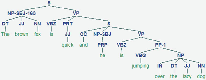
CHAPTER 3 ■ PROCESSING AND UNDERSTANDING TEXT

165

We are now able to successfully generate the parse tree for our sample sentence.

You can see the visual representation of the tree in Figure

3-7 . Remember that this is a

probabilistic PCFG parser , and you can see the overall probability of this tree mentioned

in the output earlier when we printed our parse tree. The notations of the tags followed

here are all based on the Treebank annotations we discussed earlier. Thus this shows how

to build our own constituency-based parser.

Summary

Congratulations on reaching the end of this chapter. We have covered a major chunk

of concepts, techniques, and implementations with regard to text processing, syntactic

analysis, and understanding. A lot of the concepts from Chapter

1 should seem more

relevant and clearer now that we have actually implemented them on real examples.

The content covered in this chapter is two-fold. We looked at concepts related to

text processing and normalization. You now know the importance of processing and

normalizing text, and as we move on to future chapters, you will see why it becomes

more and more important to have well-processed and standardized textual data. We

have covered various concepts and implemented techniques for text tokenization and

normalization. These include cleaning and correcting text entities like spelling and

contractions. We also built our own spelling corrector and contraction expander in the

same context. We found out a way to leverage WordNet and correct words with repeated

characters. Finally, we looked at various stemming and lemmatization concepts and

techniques. The next part of our chapter was dedicated to analyzing and understanding

text syntax and structure, where we revisited concepts from Chapter

1 including POS

tagging, shallow parsing, dependency parsing, and constituency parsing.

You now know how to use taggers and parsers on real-world textual data and ways

to implement your own taggers and parsers. We will be diving more into analyzing and

deriving insights from text in the future chapters using various ML techniques, including

classification, clustering, and summarization.

Figure 3-7. Constituency parse tree for our sample sentence based on Treebank

annotations

167

D. Sarkar, Text Analytics with Python, DOI 10.1007/978-1-4842-2388-8_4

CHAPTER 4

Text Classification

Learning to process and understand text is one of the first steps on the journey to

getting meaningful insights from textual data. Though it is important to understand

how language is structured and specific text syntax patterns, that alone is not sufficient

to be of much use to businesses and organizations who want to derive useful patterns

and insights and get maximum use out of their vast volumes of text data. Knowledge of

language processing coupled with concepts from analytics and machine learning (ML)

help in building systems that can leverage text data and help solve real-world practical

problems which benefit businesses.

Various aspects of ML include supervised learning, unsupervised learning,

reinforcement learning, and more recently deep learning. Each of these concepts involves

several techniques and algorithms that can be leveraged on text data and to build self-

learning systems that do not need too much manual supervision. An ML model is a

combination of data and algorithms—you got a taste of that in Chapter 3 was we built our

own parsers and taggers. The benefit of ML is that once a model is trained, we can directly

use it on new and previously unseen data to start seeing useful insights and desired results.

One of the most relevant and challenging problems is text classification or

categorization, which involves trying to organize text documents into various categories

based on inherent properties or attributes of each text document. This is used in

various domains, including email spam identification and news categorization. The

concept may seem simple, and if you have a small number of documents, you can look

at each document and gain some idea about what it is trying to indicate. Based on

this knowledge, you can group similar documents into categories or classes. It’s more

challenging when the number of text documents to be classified increases to several

hundred thousands or millions. This is where techniques like feature extraction and

supervised or unsupervised ML come in handy. Document classification is a generic

problem not limited to text alone but also can be extended for other items like music,

images, video, and other media.

To formalize our problem more clearly, we will have a given set of classes or

categories and several text documents. Remember that documents are basically sentences

or paragraphs of text. This forms a corpus. Our task would be to determine which class

or classes each document belongs to. This entire process involves several steps which

we will be discussing in detail later in this chapter. Briefly, for a supervised classification

problem, we need to have some labelled data that we could use for training a text

classification model. This data would essentially be curated documents that are already

assigned to some specific class or category beforehand. Using this, we would essentially

Chapter 4 ■ text ClassifiCation

168

extract features and attributes from each document and make our model learn these

attributes corresponding to each particular document and its class/category by feeding

it to a supervised ML algorithm. Of course, the data would need to be pre-processed and

normalized before building the model. Once done, we would follow the same process of

normalization and feature extraction and then feed it to the model to predict the class or

category for new documents. However, for an unsupervised classification problem, we

would essentially not have any pre-labelled training documents. We would use techniques

like clustering and document similarity measures to cluster documents together based on

their inherent properties and assign labels to them.

In this chapter, we will discuss the concept of text classification and how it can be

formulated as a supervised ML problem. We will also talk about the various forms of

classification and what they indicate. A clear depiction for the essential steps necessary

to complete a text classification workflow will also be presented, and we will be covering

some of the essential steps from the same workflow, which have not been discussed

before, including feature extraction, classifiers, model evaluation, and finally we will put

them all together in building a text classification system on real-world data.

What Is Text Classification?

Before we define text classification, we need to understand the scope of textual data and

what we really mean by classification. The textual data involved here can be anything

ranging from a phrase, sentence, or a complete document with paragraphs of text, which

can be obtained from corpora, blogs, or anywhere from the Web. Text classification is

also often called document classification just to cover all forms of textual content under

the word document. The word document could be defined as some form of concrete

representation of thoughts or events that could be in the form of writing, recorded

speech, drawings, or presentations. I use the term document here to represent textual

data such as sentences or paragraphs belonging to the English language.

Text classification is also often called text categorization, although I explicitly use

the word classification here for two reasons. First, it depicts the same essence as text

categorization, where we want to classify documents. The second reason is to also show

that we would be using classification or a supervised ML approach here to classify or

categorize the text. Text categorization can be done in many ways, as mentioned. We

will be focusing explicitly on a supervised approach using classification. The process of

classification is not restricted to text alone. It is used quite frequently in other domains

including science, healthcare, weather forecasting, and technology.

Text or document classification is the process of assigning text documents into one

or more classes or categories, assuming that we have a predefined set of classes.

Documents here are textual documents, and each document can contain a sentence or

even a paragraph of words. A text classification system would successfully be able to

classify each document to its correct class(es) based on inherent properties of the

document. Mathematically, we can define it like this: given some description and

attributes d for a document D, where

dDÎ

, and we have a set of predefined classes or

categories,

Cccc c

n

=¼

{}

12 3

, ,,, . The actual document D can have many inherent

properties and attributes that lead it to being an entity in a high-dimensional space. Using

a subset of that space with a limit set of descriptions and features depicted by d, we

Chapter 4 ■ text ClassifiCation

169

should be able to successfully assign the original document D to its correct class C

x

using

a text classification system T. This can be represented by

TD C

x

:

®

.

We will talk more about the text classification system in detail later in the chapter.

Figure4-1 shows a high-level conceptual representation of the text classification process.

In Figure4-1, we can see there are several documents representing products which

can be assigned to various categories of food, mobile phones, and movies. Initially,

these documents are all present together, just as a text corpus has various documents in

it. Once it goes through a text classification system, represented as a black box here, we

can see that each document is assigned to one specific class or category we had defined

previously. Here the documents are just represented by their names, but in real data, they

can contain much more, including descriptions of each product, specific attributes such

as movie genre, product specifications, constituents, and many more properties that can

be used as features in the text classification system to make document identification and

classification easier.

There are various types of text classification. This chapter focuses on two major

types, which are based on the type of content that makes up the documents:

• Content-based classification

• Request-based classification

Both types are more like different philosophies or ideals behind approaches to

classifying text documents rather than specific technical algorithms or processes. Content-

based classification is the type of text classification where priorities or weights are given

to specific subjects or topics in the text content that would help determine the class of the

document. A conceptual example would be that a book with more than 30 percent of its

content about food preparations can be classified under cooking/recipes. Request-based

classification is influenced by user requests and is targeted towards specific user groups

and audiences. This type of classification is governed by specific policies and ideals.

Figure 4-1. Conceptual overview of text classification

Chapter 4 ■ text ClassifiCation

170

Automated Text Classification

We now have an idea of the definition and scope of text classification. We have also

formally defined text classification both conceptually and mathematically, where we

talked about a “text classification system” being able to classify text documents to their

respective categories or classes. Consider several humans doing the task of going through

each document and classifying it. They would then be a part of the text classification

system we are talking about. However, that would not scale very well once there were

millions of text documents to be classified quickly. To make the process more efficient

and faster, we can consider automating the task of text classification, which brings us to

automated text classification.

To automate text classification, we can make use of several ML techniques and

concepts. There are mainly two types of ML techniques that are relevant to solving this

problem:

• Supervised machine learning

• Unsupervised machine learning

Besides these two techniques, there are also other families of learning algorithms,

such as reinforcement learning and semi-supervised learning. Let us look at both

supervised and unsupervised learning algorithms in more detail, from both an ML

perspective how it can be leveraged in classifying text documents.

Unsupervised learning refers to specific ML techniques or algorithms that do not

require any pre-labelled training data samples to build a model. We usually have a

collection of data points, which could be text or numeric, depending on the problem we

are trying to solve. We extract features from each of the data points using a process known

as feature extraction and then feed the feature set for each data point into our algorithm.

We are trying to extract meaningful patterns from the data, such as trying to group

together similar data points using techniques like clustering or summarizing documents

based on topic models. This is extremely useful in text document categorization and is

also called document clustering, where we cluster documents into groups purely based

on their features, similarity, and attributes, without training any model on previously

labelled data. Later chapters further discuss unsupervised learning, covering topic

models, document summarization, similarity analysis, and clustering.

Supervised learning refers to specific ML techniques or algorithms that are trained

on pre-labelled data samples known as training data. Features or attributes are extracted

from this data using feature extraction, and for each data point we will have its own

feature set and corresponding class/label. The algorithm learns various patterns for each

type of class from the training data. Once this process is complete, we have a trained

model. This model can then be used to predict the class for future test data samples once

we feed their features to the model. Thus the machine has actually learned, based on

previous training data samples, how to predict the class for new unseen data samples.

There are two major types of supervised learning algorithms:

• Classification: The process of supervised learning is referred to

as classification when the outcomes to be predicted are distinct

categories, thus the outcome variable is a categorical variable in

this case. Examples would be news categories or movie genres.

Chapter 4 ■ text ClassifiCation

171

• Regression: Supervised learning algorithms are known as

regression algorithms when the outcome we want to predict is a

continuous numeric variable. Examples would be house prices or

people’s weights.

We will be specifically focusing on classification for our problem (hence the name of

the chapter—we are trying to classify or categorize text documents into distinct classes or

categories. We will be following a supervised learning approach in our implementations

later on.

Now we are ready to define the process of automated or ML-based text classification

mathematically. Say we have a training set of documents labelled with their corresponding

class or category. This can be represented by TS, which is a set of paired documents and

labels,

TS dc dc dc

nn

=

()()

¼

()

{}

11 22,, ,

,,, where d

1

,d

2

,…,d

n

is the list of text documents,

and their corresponding labels are c

1

,c

2

,…,c

n

such that cCcc cn

x

Î= ¼

{}

12,,, where c

x

denotes the class label for document x and C denotes the set of all possible distinct classes,

any of which can be the class or classes for each document. Assuming we have our training

set, we can define a supervised learning algorithm F such that when it is trained on our

training dataset TS, we build a classification model or classifier γ such that we can say

that

FTS

()

=

g

. Thus the supervised learning algorithm F takes the input set of (document,

class) pairs TS and gives us the trained classifier γ, which is our model. This process is

known as the training process.

This model can then take a new, previously unseen document ND and predict its

class c

ND

such that

cC

ND

Î

. This process is known as the prediction process and can be

represented by

g

:TD c

ND

®

. Thus we can see that there are two main processes in the

supervised text classification process:

• Training

• Prediction

An important point to remember is that some manually labelled training data

is necessary for supervised text classification, so even though we are talking about

automated text classification, to kick start the process we need some manual efforts. Of

course, the benefits of this are manifold because once we have a trained classifier, we can

keep using it to predict and classify new documents with minimal efforts and manual

supervision.

There are various learning methods or algorithms that we will be discussing in a

future section. These learning algorithms are not specific to text data but are generic ML

algorithms that can be applied toward various types of data after due pre-processing

and feature extraction. I will touch upon a couple of supervised ML algorithms and use

them in solving a real-world text classification problem. These algorithms are usually

trained on the training data set and often an optional validation set such that the model

that is trained does not overfit to the training data, which basically means it would then

not be able to generalize well and predict properly for new instances of text documents.

Often the model is tuned on several of its internal parameters based on the learning

algorithm and by evaluating various performance metrics like accuracy on the validation

set or by using cross-validation where we split the training dataset itself into training and

Chapter 4 ■ text ClassifiCation

172

validation sets by random sampling. This comprises the training process, the outcome

of which yields a fully trained model that is ready to predict. In the prediction stage,

we usually have new data points from the test dataset. We can use them to feed into

the model after normalization and feature extraction and see how well the model is

performing by evaluating its prediction performance.

There are a few types of text classification based on the number of classes to predict

and the nature of predictions. These types of classification are based on the dataset, the

number of classes/categories pertaining to that dataset, and the number of classes that

can be predicted on any data point:

• Binary classification is when the total number of distinct classes

or categories is two in number and any prediction can contain

either one of those classes.

• Multi-class classification, also known as multinomial

classification, refers to a problem where the total number of

classes is more than two, and each prediction gives one class

or category that can belong to any of those classes. This is an

extension of the binary classification problem where the total

number of classes is more than two.

• Multi-label classification refers to problems where each prediction

can yield more than one outcome/predicted class for any data

point.

Text Classification Blueprint

Now that we know the basic scope of automated text classification, this section will look

at a blueprint for a complete workflow of building an automated text classifier system.

This will consist of a series of steps that must be followed in both the training and testing

phases mentioned in the earlier section. For building a text classification system, we

need to make sure we have our source of data and retrieve that data so that we can start

feeding it to our system. The following main steps outline a typical workflow for a text

classification system, assuming we have our datasetalready downloaded and ready to

be used:

1. Prepare train and test datasets

2. Text normalization

3. Feature extraction

4. Model training

5. Model prediction and evaluation

6. Model deployment

These steps are carried out in that order for building a text classifier. Figure4-2 shows

a detailed workflow for a text classification system with the main processes highlighted in

training and prediction.

Chapter 4 ■ text ClassifiCation

173

Notice that there are two main boxes for Training and Prediction, which are the

two main processes involved in building a text classifier. In general, the dataset we have

is usually divided into two or three splits called the training, validation (optional), and

testing datasets, respectively. You can see an overlap of the Text Normalization and Feature

Extraction modules in Figure4-2 for both processes, indicating that no matter which

document we want to classify and predict its class, it must go through the same series

of transformations in both the training and prediction process. Each document is first

pre-processed and normalized, and then specific features pertaining to the document are

extracted. These processes are always uniform in both the training and prediction processes

to make sure that our classification model performs consistently in its predictions.

In the Training process, each document has its own corresponding class/category

that was manually labeled or curated beforehand. These training text documents are

processed and normalized in the Text Normalization module, giving us clean and

standardized training text documents. They are then passed to the Feature Extraction

module where different types of feature-extraction techniques are used to extract

meaningful features from the processed text documents. We will cover some popular

feature extraction techniques in a future section. These features are usually numeric

arrays or vectors because standard ML algorithms work on numeric vectors. Once we

have our features, we select a supervised ML algorithm and train our model.

Training the model involves feeding the feature vectors for the documents and

the corresponding labels such that the algorithm is able to learn various patterns

corresponding to each class/category and can reuse this learned knowledge to predict

classes for future new documents. Often an optional validation dataset is used to evaluate

the performance of the classification algorithm to make sure it generalizes well with

the data during training. A combination of these features and the ML algorithm yields a

Classification Model, which is the end stage of the Training process. Often this model is

tuned using various model parameters with a process called hyperparameter tuning to

build a better performing optimal model.

Figure 4-2. Blueprint for building an automated text classification system

Chapter 4 ■ text ClassifiCation

174

The Prediction process shown in the figure involves trying to either predict classes

for new documents or evaluating how predictions are working on testing data. The test

dataset documents go through the same process of normalization and feature extraction,

and the test document features are passed to the trained Classification Model, which

predicts the possible class for each of the documents based on previously learned

patterns. If you have the true class labels for the documents that were manually labelled,

you can evaluate the prediction performance of the model by comparing the true labels

and the predicted labels using various metrics like accuracy. This would give an idea of

how well the model performs its predictions for new documents.

Once we have a stable and working model, the last step is usually deploying the

model, which normally involves saving the model and its necessary dependencies

and deploying it as a service or as a running program that predicts categories for new

documents as a batch job, or based on serving user requests if accessed as a web service.

There are various ways to deploy ML models, and this usually depends on how you want

to access it later on.

We will now discuss some of the main modules from the preceding blueprint and

implement these modules so that we can integrate them all together to build a real-world

text classifier.

Text Normalization

Chapter 3 covered text processing and normalization in detail—refer it to see the various

methods and techniques available. In this section, we will define a normalizer module to

normalize text documents and will be using it later when we build our classifier. Although

various techniques are available, we will keep it fairly simple and straightforward here so

that is it not too hard to follow our implementations step by step. We will implement and

use the following normalization techniques in our module:

• Expanding contractions

• Text standardization through lemmatization

• Removing special characters and symbols

• Removing stopwords

We are not focusing too much on correcting spellings and other advanced

techniques, but you can integrate the functions from the previous chapter

implementation if you are interested. Our normalization module is implemented and

available in normalization.py, available in the code files for this chapter. I will also be

explaining each function here for your convenience. We will first start with loading the

necessary dependencies. Remember that you will need our custom-defined contractions

mapping file from Chapter 3, named contractions.py, for expanding contractions.

The following snippet shows the necessary imports and dependencies:

from contractions import CONTRACTION_MAP

import re

import nltk

import string

from nltk.stem import WordNetLemmatizer

Chapter 4 ■ text ClassifiCation

175

stopword_list = nltk.corpus.stopwords.words('english')

wnl = WordNetLemmatizer()

We load all the English stopwords, the contraction mappings in CONTRACTION_MAP,

and an instance of WordNetLemmatizer for carrying our lemmatization. We now define

a function to tokenize text into tokens that will be used by our other normalization

functions. The following function tokenizes and removes any extraneous whitespace from

the tokens:

def tokenize_text(text):

tokens = nltk.word_tokenize(text)

tokens = [token.strip() for token in tokens]

return tokens

Now we define a function for expanding contractions. This function is similar to our

implementation from Chapter 3—it takes in a body of text and returns the same with its

contractions expanded if there is a match. The following snippet helps us achieve this:

def expand_contractions(text, contraction_mapping):

contractions_pattern = re.compile('({})'.format('|'.join(contraction_

mapping.keys())),

flags=re.IGNORECASE|re.DOTALL)

def expand_match(contraction):

match = contraction.group(0)

first_char = match[0]

expanded_contraction = contraction_mapping.get(match)\

if contraction_mapping.get(match)\

else contraction_mapping.get(match.lower())

expanded_contraction = first_char+expanded_contraction[1:]

return expanded_contraction

expanded_text = contractions_pattern.sub(expand_match, text)

expanded_text = re.sub("'", "", expanded_text)

return expanded_text

Now that we have a function for expanding contractions, we implement a function

for standardizing our text data by bringing word tokens to their base or root form using

lemmatization. The following functions will help us in achieving that:

from pattern.en import tag

from nltk.corpus import wordnet as wn

# Annotate text tokens with POS tags

def pos_tag_text(text):

# convert Penn treebank tag to wordnet tag

Chapter 4 ■ text ClassifiCation

176

def penn_to_wn_tags(pos_tag):

if pos_tag.startswith('J'):

return wn.ADJ

elif pos_tag.startswith('V'):

return wn.VERB

elif pos_tag.startswith('N'):

return wn.NOUN

elif pos_tag.startswith('R'):

return wn.ADV

else:

return None

tagged_text = tag(text)

tagged_lower_text = [(word.lower(), penn_to_wn_tags(pos_tag))

for word, pos_tag in

tagged_text]

return tagged_lower_text

# lemmatize text based on POS tags

def lemmatize_text(text):

pos_tagged_text = pos_tag_text(text)

lemmatized_tokens = [wnl.lemmatize(word, pos_tag) if pos_tag

else word

for word, pos_tag in pos_tagged_text]

lemmatized_text = ' '.join(lemmatized_tokens)

return lemmatized_text

The preceding snippet depicts two functions implemented for lemmatization. The

main function is lemmatize_text, which takes in a body of text data and lemmatizes

each word of the text based on its POS tag if it is present and then returns the lemmatized

text back to the user. For this, we need to annotate the text tokens with their POS tags.

We use the tag function from pattern to annotate POS tags for each token and then

further convert the POS tags from the Penn treebank syntax to WordNet syntax, since

the WordNetLemmatizer checks for POS tag annotations based on WordNet formats. We

convert each word token to lowercase, annotate it with its correct, converted WordNet

POS tag, and return these annotated tokens, which are finally fed into the lemmatize_

text function.

The following function helps us remove special symbols and characters:

def remove_special_characters(text):

tokens = tokenize_text(text)

pattern = re.compile('[{}]'.format(re.escape(string.punctuation)))

filtered_tokens = filter(None, [pattern.sub('', token) for token in

tokens])

filtered_text = ' '.join(filtered_tokens)

return filtered_text

Chapter 4 ■ text ClassifiCation

177

We remove special characters by tokenizing the text just so we can remove some of

the tokens that are actually contractions, but we may have failed to remove them in our

first step, like "s" or "re". We will do this when we remove stopwords. However, you can

also remove special characters without tokenizing the text. We remove all special symbols

defined in string.punctuation from our text using regular expression matches. The

following function helps us remove stopwords from our text data:

def remove_stopwords(text):

tokens = tokenize_text(text)

filtered_tokens = [token for token in tokens if token not in

stopword_list]

filtered_text = ' '.join(filtered_tokens)

return filtered_text

Now that we have all our functions defined, we can build our text normalization

pipeline by chaining all these functions one after another. The following function

implements this, where it takes in a corpus of text documents and normalizes them and

returns a normalized corpus of text documents:

def normalize_corpus(corpus, tokenize=False):

normalized_corpus = []

for text in corpus:

text = expand_contractions(text, CONTRACTION_MAP)

text = lemmatize_text(text)

text = remove_special_characters(text)

text = remove_stopwords(text)

normalized_corpus.append(text)

if tokenize:

text = tokenize_text(text)

normalized_corpus.append(text)

return normalized_corpus

That brings us to the end of our discussion and implementation of necessary

functions for our text normalization module. We will now look at concepts and practical

implementation for feature extraction.

Feature Extraction

There are various feature-extraction techniques that can be applied on text data, but

before we jump into then, let us consider what we mean by features. Why do we need

them, and how they are useful? In a dataset, there are typically many data points. Usually

the rows of the dataset and the columns are various features or properties of the dataset,

with specific values for each row or observation. In ML terminology, features are unique,

measurable attributes or properties for each observation or data point in a dataset.

Features are usually numeric in nature and can be absolute numeric values or categorical

Chapter 4 ■ text ClassifiCation

178

features that can be encoded as binary features for each category in the list using a

process called one-hot encoding. The process of extracting and selecting features is both

art and science, and this process is called feature extraction or feature engineering.

Usually extracted features are fed into ML algorithms for learning patterns that can

be applied on future new data points for getting insights. These algorithms usually expect

features in the form of numeric vectors because each algorithm is at heart a mathematical

operation of optimization and minimizing loss and error when it tries to learn patterns

from data points and observations. So, with textual data there is the added challenge of

figuring out how to transform textual data and extract numeric features from it.

Now we will look at some feature-extraction concepts and techniques specially

aligned towards text data.

The Vector Space Model is a concept and model that is very useful in case we are

dealing with textual data and is very popular in information retrieval and document

ranking. The Vector Space Model, also known as the Term Vector Model, is defined as a

mathematical and algebraic model for transforming and representing text documents as

numeric vectors of specific terms that form the vector dimensions. Mathematically this

can be defines as follows. Say we have a document D in a document vector space VS. The

number of dimensions or columns for each document will be the total number of distinct

terms or words for all documents in the vector space. So, the vector space can be denoted

VS WW W

n

=¼

{}

12

,,,

where there are n distinct words across all documents. Now we can represent document

D in this vector space as

Dw

ww

DD Dn

=¼

{}

12

,,,

where w

Dn

denotes the weight for word n in document D. This weight is a numeric value

and can represent anything, ranging from the frequency of that word in the document, to

the average frequency of occurrence, or even to the TF-IDF weight (discussed shortly).

We will be talking about and implementing the following feature-extraction

techniques:

• Bag of Words model

• TF-IDF model

• Advanced word vectorization models

An important thing to remember for feature extraction is that once we build a

feature extractor using some transformations and mathematical operations, we need to

make sure we reuse the same process when extracting features from new documents to

be predicted, and not rebuild the whole algorithm again based on the new documents.

We will be depicting this also with an example for each technique. Do note that for

implementations based on practical examples in this section, we will be making use

of the nltk, gensim, and scikit-learn libraries, which you can install using pip as

discussed earlier (in case you do not have them installed already).

Chapter 4 ■ text ClassifiCation

179

The implementations are divided into two major modules. The file feature_

extractors.py contains the generic functions we will be using later on when building the

classifier, and we have used the same functions in the feature_extraction_demo.py file to

show how each technique works with some practical examples. You can access them from

the code files, and as always I will be presenting the same code in this chapter for ease of

understanding. We will be using the following documents depicted in the CORPUS variable

to extract features from and building some of the vectorization models. To illustrate how

feature extraction will work for a new document (as a part of test dataset), we will also use

a separate document as shown in the variable new_doc in the following snippet:

CORPUS = [

'the sky is blue',

'sky is blue and sky is beautiful',

'the beautiful sky is so blue',

'i love blue cheese'

]

new_doc = ['loving this blue sky today']

Bag of Words Model

The Bag of Words model is perhaps one of the simplest yet most powerful techniques

to extract features from text documents. The essence of this model is to convert text

documents into vectors such that each document is converted into a vector that

represents the frequency of all the distinct words that are present in the document

vector space for that specific document. Thus, considering our sample vector from the

previous mathematical notation for D, the weight for each word is equal to its frequency

of occurrence in that document.

An interesting thing is that we can even create the same model for individual word

occurrences as well as occurrences for n-grams, which would make it an n-gram Bag of

Words model such that frequency of distinct n-grams in each document would also be

considered.

The following code snippet gives us a function that implements a Bag of Words–

based feature-extraction model that also accepts an ngram_range parameter to take into

account n-grams as features:

from sklearn.feature_extraction.text import CountVectorizer

def bow_extractor(corpus, ngram_range=(1,1)):

vectorizer = CountVectorizer(min_df=1, ngram_range=ngram_range)

features = vectorizer.fit_transform(corpus)

return vectorizer, features

The preceding function uses the CountVectorizer class. You can access its detailed

API (Application Programming Interface) documentation at http://scikit-learn.org/

stable/modules/generated/sklearn.feature_extraction.text.CountVectorizer.

Chapter 4 ■ text ClassifiCation

180

html#sklearn.feature_extraction.text.CountVectorizer, which has a whole bunch

of various parameters for more fine-tuning based on the type of features you want to

extract. We use its default configuration, which is enough for most scenarios, with min_df

set to 1 indicating taking terms having a minimum frequency of 1 in the overall document

vector space. You can set ngram_range to various parameters like (1, 3) would build

feature vectors consisting of all unigrams, bigrams, and trigrams. The following snippet

shows the function in action on our sample corpora of four training documents and one

test document:

# build bow vectorizer and get features

In [371]: bow_vectorizer, bow_features = bow_extractor(CORPUS)

...: features = bow_features.todense()

...: print features

[[0 0 1 0 1 0 1 0 1]

[1 1 1 0 2 0 2 0 0]

[0 1 1 0 1 0 1 1 1]

[0 0 1 1 0 1 0 0 0]]

# extract features from new document using built vectorizer

In [373]: new_doc_features = bow_vectorizer.transform(new_doc)

...: new_doc_features = new_doc_features.todense()

...: print new_doc_features

[[0 0 1 0 0 0 1 0 0]]

# print the feature names

In [374]: feature_names = bow_vectorizer.get_feature_names()

...: print feature_names

[u'and', u'beautiful', u'blue', u'cheese', u'is', u'love', u'sky', u'so',

u'the']

That output shows how each text document has been converted to vectors. Each row

represents one document from our corpus, and we do the same for both our corpora. The

vectorizer is built using documents from CORPUS. We extract features from it and also use

this built vectorizer to extract features from a completely new document. Each column in

a vector represents the words depicted in feature_names, and the value is the frequency

of that word in the document represented by the vector. It may be hard to comprehend

this at first glance, so I have prepared the following function, which I hope you can use to

understand the feature vectors better:

import pandas as pd

def display_features(features, feature_names):

df = pd.DataFrame(data=features,

columns=feature_names)

print df

Now you can feed the feature names and vectors to this function and see the feature

matrix in a much easier-to-understand structure, shown here:

Chapter 4 ■ text ClassifiCation

181

In [379]: display_features(features, feature_names)

and beautiful blue cheese is love sky so the

0 0 0 1 0 1 0 1 0 1

1 1 1 1 0 2 0 2 0 0

2 0 1 1 0 1 0 1 1 1

3 0 0 1 1 0 1 0 0 0

In [380]: display_features(new_doc_features, feature_names)

and beautiful blue cheese is love sky so the

0 0 0 1 0 0 0 1 0 0

That makes things much clearer, right? Consider the second document of CORPUS,

represented in the preceding in row 1 of the first table. You can see that 'sky is blue

and sky is beautiful' has value 2 for the feature sky, 1 for beautiful, and so on.

Values of 0 are assigned for words not present in the document. Note that for the new

document new_doc, there is no feature for the words today, this, or loving in the

sentence. The reason for this is what I mentioned before—that the feature-extraction

process, model, and vocabulary are always based on the training data and will never

change or get influenced on newer documents, which it will predict later as a part of

testing or otherwise. You might have guessed that this is because a model is always

trained on some training data and is never influenced by newer documents unless we

plan on rebuilding that model. Hence, the features in this model are always limited based

on the document vector space of the training corpus.

You have now started to get an idea of how to extract meaningful vector-based

features from text data, which previously seemed impossible. Try out the preceding

functions by setting ngram_range to (1, 3) and see the outputs.

TF-IDF Model

The Bag of Words model is good, but the vectors are completely based on absolute

frequencies of word occurrences. This has some potential problems where words that

may tend to occur a lot across all documents in the corpus will have higher frequencies

and will tend to overshadow other words that may not occur as frequently but may

be more interesting and effective as features to identify specific categories for the

documents. This is where TF-IDF comes into the picture. TF-IDF stands for Term

Frequency-Inverse Document Frequency, a combination of two metrics: term frequency

and inverse document frequency. This technique was originally developed as a metric for

ranking functions for showing search engine results based on user queries and has come

to be a part of information retrieval and text feature extraction now.

Let us formally define TF-IDF now and look at the mathematical representations for

it before diving into its implementation. Mathematically, TF-IDF is the product of two

metrics and can be represented as

tfidftfidf

=´

, where term frequency (tf) and

inverse-document frequency (idf) represent the two metrics.

Term frequency denoted by tf is what we had computed in the Bag of Words model.

Term frequency in any document vector is denoted by the raw frequency value of that

term in a particular document. Mathematically it can be represented as

tf wD f

w

D

,

()

= ,

where

f

w

D

denotes frequency for word w in document D, which becomes the term

Chapter 4 ■ text ClassifiCation

182

frequency (tf). There are various other representations and computations for term

frequency, such as converting frequency to a binary feature where 1 means the term has

occurred in the document and 0 means it has not. Sometimes you can also normalize the

absolute raw frequency using logarithms or averaging the frequency. We will be using the

raw frequency in our computations.

Inverse document frequency denoted by idf is the inverse of the document frequency

for each term. It is computed by dividing the total number of documents in our corpus

by the document frequency for each term and then applying logarithmic scaling on the

result. In our implementation we will be adding 1 to the document frequency for each

term just to indicate that we also have one more document in our corpus that essentially

has every term in the vocabulary. This is to prevent potential division-by-zero errors

and smoothen the inverse document frequencies. We also add 1 to the result of our idf

computation to avoid ignoring terms completely that might have zero idf. Mathematically

our implementation for idf can be represented by

idft

C

df t

()

=+

+

()

1

log

where idf(t) represents the idf for the term t, C represents the count of the total number of

documents in our corpus, and df(t) represents the frequency of the number of documents

in which the term t is present.

Thus the term frequency-inverse document frequency can be computed by

multiplying the above two measures together. The final TF-IDF metric we will be using is

a normalized version of the tfidf matrix we get from the product of tf and idf. We will

normalize the tfidf matrix by dividing it with the L2 norm of the matrix, also known as the

Euclidean norm, which is the square root of the sum of the square of each term’s tfidf

weight. Mathematically we can represent the final tfidf feature vector as

tfidf

=

,

where

tfidf

represents the Euclidean L2 norm for the tfidf matrix.

The following code snippet shows an implementation of getting the tfidf-based

feature vectors, considering we have our Bag of Words feature vectors we obtained in the

previous section:

from sklearn.feature_extraction.text import TfidfTransformer

def tfidf_transformer(bow_matrix):

transformer = TfidfTransformer(norm='l2',

smooth_idf=True,

use_idf=True)

tfidf_matrix = transformer.fit_transform(bow_matrix)

return transformer, tfidf_matrix

You can see that we have used the L2 norm option in the parameters and also made

sure we smoothen the idfs to give weightages also to terms that may have zero idf so that

we do not ignore them. We can see this function in action in the following code snippet:

Chapter 4 ■ text ClassifiCation

183

import numpy as np

from feature_extractors import tfidf_transformer

feature_names = bow_vectorizer.get_feature_names()

# build tfidf transformer and show train corpus tfidf features

In [388]: tfidf_trans, tdidf_features = tfidf_transformer(bow_features)

...: features = np.round(tdidf_features.todense(), 2)

...: display_features(features, feature_names)

and beautiful blue cheese is love sky so the

0 0.00 0.00 0.40 0.00 0.49 0.00 0.49 0.00 0.60

1 0.44 0.35 0.23 0.00 0.56 0.00 0.56 0.00 0.00

2 0.00 0.43 0.29 0.00 0.35 0.00 0.35 0.55 0.43

3 0.00 0.00 0.35 0.66 0.00 0.66 0.00 0.00 0.00

# show tfidf features for new_doc using built tfidf transformer

In [389]: nd_tfidf = tfidf_trans.transform(new_doc_features)

...: nd_features = np.round(nd_tfidf.todense(), 2)

...: display_features(nd_features, feature_names)

and beautiful blue cheese is love sky so the

0 0.0 0.0 0.63 0.0 0.0 0.0 0.77 0.0 0.0

Thus the preceding outputs show the tfidf feature vectors for all our sample

documents. We use the TfidfTransformer class, which helps us in computing the tfidfs

for each document based on the equations described earlier.

Now we will show how the internals of this class work. You will also see how to

implement the mathematical equations described earlier to compute the tfidf-based

feature vectors. This section is dedicated to ML experts (and curious readers who are

interested in how things work behind the scenes). We will start with loading necessary

dependencies and computing the term frequencies (TF) by reusing our Bag of Words-

based features for our sample corpus, which can also act as the term frequencies for our

training CORPUS:

import scipy.sparse as sp

from numpy.linalg import norm

feature_names = bow_vectorizer.get_feature_names()

# compute term frequency

tf = bow_features.todense()

tf = np.array(tf, dtype='float64')

# show term frequencies

In [391]: display_features(tf, feature_names)

and beautiful blue cheese is love sky so the

0 0.0 0.0 1.0 0.0 1.0 0.0 1.0 0.0 1.0

1 1.0 1.0 1.0 0.0 2.0 0.0 2.0 0.0 0.0

2 0.0 1.0 1.0 0.0 1.0 0.0 1.0 1.0 1.0

3 0.0 0.0 1.0 1.0 0.0 1.0 0.0 0.0 0.0

Chapter 4 ■ text ClassifiCation

184

We will now compute our document frequencies (DF) for each term based on the

number of documents in which it occurs. The following snippet shows how to obtain it

from our Bag of Words feature matrix:

# build the document frequency matrix

df = np.diff(sp.csc_matrix(bow_features, copy=True).indptr)

df = 1 + df # to smoothen idf later

# show document frequencies

In [403]: display_features([df], feature_names)

and beautiful blue cheese is love sky so the

0 2 3 5 2 4 2 4 2 3

This tells us the document frequency (DF) for each term and you can verify it with

the documents in CORPUS. Remember that we have added 1 to each frequency value to

smoothen the idf values later and prevent division-by-zero errors by assuming we have a

document (imaginary) that has all the terms once. Thus, if you check in the CORPUS, you

will see that blue occurs 4(+1) times, sky occurs 3(+1) times, and so on, considering (+1)

for our smoothening.

Now that we have the document frequencies, we will compute the inverse document

frequency (idf) using our formula defined earlier. Remember to add 1 to the total count of

documents in the corpus to add the document that we had assumed earlier to contain all

the terms at least once for smoothening the idfs:

# compute inverse document frequencies

total_docs = 1 + len(CORPUS)

idf = 1.0 + np.log(float(total_docs) / df)

# show inverse document frequencies

In [406]: display_features([np.round(idf, 2)], feature_names)

and beautiful blue cheese is love sky so the

0 1.92 1.51 1.0 1.92 1.22 1.92 1.22 1.92 1.51

# compute idf diagonal matrix

total_features = bow_features.shape[1]

idf_diag = sp.spdiags(idf, diags=0, m=total_features, n=total_features)

idf = idf_diag.todense()

# print the idf diagonal matrix

In [407]: print np.round(idf, 2)

[[ 1.92 0. 0. 0. 0. 0. 0. 0. 0. ]

[ 0. 1.51 0. 0. 0. 0. 0. 0. 0. ]

[ 0. 0. 1. 0. 0. 0. 0. 0. 0. ]

[ 0. 0. 0. 1.92 0. 0. 0. 0. 0. ]

[ 0. 0. 0. 0. 1.22 0. 0. 0. 0. ]

[ 0. 0. 0. 0. 0. 1.92 0. 0. 0. ]

[ 0. 0. 0. 0. 0. 0. 1.22 0. 0. ]

[ 0. 0. 0. 0. 0. 0. 0. 1.92 0. ]

[ 0. 0. 0. 0. 0. 0. 0. 0. 1.51]]

Chapter 4 ■ text ClassifiCation

185

You can now see the idf matrix that we created based on our mathematical equation,

and we also convert it to a diagonal matrix, which will be helpful later on when we want

to compute the product with term frequency.

Now that we have our tfs and idfs, we can compute the tfidf feature matrix using

matrix multiplication, as shown in the following snippet:

# compute tfidf feature matrix

tfidf = tf * idf

# show tfidf feature matrix

In [410]: display_features(np.round(tfidf, 2), feature_names)

and beautiful blue cheese is love sky so the

0 0.00 0.00 1.0 0.00 1.22 0.00 1.22 0.00 1.51

1 1.92 1.51 1.0 0.00 2.45 0.00 2.45 0.00 0.00

2 0.00 1.51 1.0 0.00 1.22 0.00 1.22 1.92 1.51

3 0.00 0.00 1.0 1.92 0.00 1.92 0.00 0.00 0.00

We now have our tfidf feature matrix, but wait! It is not yet over. We have to divide it

with the L2 norm, if you remember from our equations depicted earlier. The following

snippet computes the tfidf norms for each document and then divides the tfidf weights

with the norm to give us the final desired tfidf matrix:

# compute L2 norms

norms = norm(tfidf, axis=1)

# print norms for each document

In [412]: print np.round(norms, 2)

[ 2.5 4.35 3.5 2.89]

# compute normalized tfidf

norm_tfidf = tfidf / norms[:, None]

# show final tfidf feature matrix

In [415]: display_features(np.round(norm_tfidf, 2), feature_names)

and beautiful blue cheese is love sky so the

0 0.00 0.00 0.40 0.00 0.49 0.00 0.49 0.00 0.60

1 0.44 0.35 0.23 0.00 0.56 0.00 0.56 0.00 0.00

2 0.00 0.43 0.29 0.00 0.35 0.00 0.35 0.55 0.43

3 0.00 0.00 0.35 0.66 0.00 0.66 0.00 0.00 0.00

Compare the preceding obtained tfidf feature matrix for the documents in CORPUS

to the feature matrix obtained using TfidfTransformer earlier. Note they are exactly the

same, thus verifying that our mathematical implementation was correct—and in fact this

very same implementation is adopted by scikit-learn’s TfidfTransformer behind the

scenes using some more optimizations. Now, suppose we want to compute the tfidf-

based feature matrix for our new document new_doc. We can do it using the following

snippet. We reuse the new_doc_features Bag of Words vector from before for the term

frequencies:

Chapter 4 ■ text ClassifiCation

186

# compute new doc term freqs from bow freqs

nd_tf = new_doc_features

nd_tf = np.array(nd_tf, dtype='float64')

# compute tfidf using idf matrix from train corpus

nd_tfidf = nd_tf*idf

nd_norms = norm(nd_tfidf, axis=1)

norm_nd_tfidf = nd_tfidf / nd_norms[:, None]

# show new_doc tfidf feature vector

In [418]: display_features(np.round(norm_nd_tfidf, 2), feature_names)

and beautiful blue cheese is love sky so the

0 0.0 0.0 0.63 0.0 0.0 0.0 0.77 0.0 0.0

The preceding output depicts the tfidf-based feature vector for new_doc, and you can

see it is the same as the one obtained by TfidfTransformer.

Now that we know how the internals work, we are going to implement a generic

function that can directly compute the tfidf-based feature vectors for documents from the

raw documents themselves. The following snippet depicts the same:

from sklearn.feature_extraction.text import TfidfVectorizer

def tfidf_extractor(corpus, ngram_range=(1,1)):

vectorizer = TfidfVectorizer(min_df=1,

norm='l2',

smooth_idf=True,

use_idf=True,

ngram_range=ngram_range)

features = vectorizer.fit_transform(corpus)

return vectorizer, features

The preceding function makes use of the TfidfVectorizer, which directly computes

the tfidf vectors by taking the raw documents themselves as input and internally

computing the term frequencies as well as the inverse document frequencies, eliminating

the need to use the CountVectorizer for computing the term frequencies based on the

Bag of Words model. Support is also present for adding n-grams to the feature vectors. We

can see the function in action in the following snippet:

# build tfidf vectorizer and get training corpus feature vectors

In [425]: tfidf_vectorizer, tdidf_features = tfidf_extractor(CORPUS)

...: display_features(np.round(tdidf_features.todense(), 2), feature_

names)

and beautiful blue cheese is love sky so the

0 0.00 0.00 0.40 0.00 0.49 0.00 0.49 0.00 0.60

1 0.44 0.35 0.23 0.00 0.56 0.00 0.56 0.00 0.00

2 0.00 0.43 0.29 0.00 0.35 0.00 0.35 0.55 0.43

3 0.00 0.00 0.35 0.66 0.00 0.66 0.00 0.00 0.00

Chapter 4 ■ text ClassifiCation

187

# get tfidf feature vector for the new document

In [426]: nd_tfidf = tfidf_vectorizer.transform(new_doc)

...: display_features(np.round(nd_tfidf.todense(), 2), feature_names)

and beautiful blue cheese is love sky so the

0 0.0 0.0 0.63 0.0 0.0 0.0 0.77 0.0 0.0

You can see from the preceding outputs that the tfidf feature vectors match to the

ones we obtained previously. This brings us to the end of our discussion on feature

extraction using tfidf. Now we will look at some advanced word vectorization techniques.

Advanced Word Vectorization Models

There are various approaches to creating more advanced word vectorization models for

extracting features from text data. Here we will discuss a couple of them that use Google’s

popular word2vec algorithm. The word2vec model, released in 2013 by Google, is a neural

network–based implementation that learns distributed vector representations of words

based on continuous Bag of Words and skip-gram–based architectures. The word2vec

framework is much faster than other neural network–based implementations and does

not require manual labels to create meaningful representations among words. You can

find more details on Google’s word2vec project at https://code.google.com/archive/p/

word2vec/. You can even try out some of the implementations yourself if you are interested.

We will be using the gensim library in our implementation, which is Python

implementation for word2vec that provides several high-level interfaces for easily building

these models. The basic idea is to provide a corpus of documents as input and get feature

vectors for them as output. Internally, it constructs a vocabulary based on the input text

documents and learns vector representations for words based on various techniques

mentioned earlier, and once this is complete, it builds a model that can be used to

extract word vectors for each word in a document. Using various techniques like average

weighting or tfidf weighting, we can compute the averaged vector representation of a

document using its word vectors. You can get more details about the interface for gensim‘s

word2vec implementation at http://radimrehurek.com/gensim/models/word2vec.html.

We will be mainly focusing on the following parameters when we build our model

from our sample training corpus:

• size: This parameter is used to set the size or dimension for the

word vectors and can range from tens to thousands. You can try

out various dimensions to see which gives the best result.

• window: This parameter is used to set the context or window size.

which specifies the length of the window of words that should be

considered for the algorithm to take into account as context when

training.

• min_count: This parameter specifies the minimum word count

needed across the corpus for the word to be considered in the

vocabulary. This helps in removing very specific words that may

not have much significance because they occur very rarely in the

documents.

Chapter 4 ■ text ClassifiCation

188

• sample: This parameter is used to downsample effects of

occurrence of frequent words. Values between 0.01 and 0.0001 are

usually ideal.

Once we build a model, we will define and implement two techniques of combining

word vectors together in text documents based on certain weighing schemes. We will

implement two techniques mentioned as follows.

• Averaged word vectors

• TF-IDF weighted word vectors

Let us start the feature-extraction process by building our word2vec model on our

sample training corpus before going into further implementations. The following code

snippet shows how:

import gensim

import nltk

# tokenize corpora

TOKENIZED_CORPUS = [nltk.word_tokenize(sentence)

for sentence in CORPUS]

tokenized_new_doc = [nltk.word_tokenize(sentence)

for sentence in new_doc]

# build the word2vec model on our training corpus

model = gensim.models.Word2Vec(TOKENIZED_CORPUS, size=10, window=10,

min_count=2, sample=1e-3)

As you can see, we have built the model using the parameters described earlier; you

can play around with these and also look at other parameters from the documentation to

change the architecture type, number of workers, and so on. Now that we have our model

ready, we can start implementing our feature extraction techniques.

Averaged Word Vectors

The preceding model creates a vector representation for each word in the vocabulary. We

can access them by just typing in the following code:

In [430]: print model['sky']

[ 0.01608407 -0.04819566 0.04227461 -0.03011346 0.0254148 0.01728328

0.0155535 0.00774884 -0.02752112 0.01646519]

In [431]: print model['blue']

[-0.0472235 0.01662185 -0.01221706 -0.04724348 -0.04384995 0.00193343

-0.03163504 -0.03423524 0.02661656 0.03033725]

Each word vector is of length 10 based on the size parameter specified earlier. But

when we deal with sentences and text documents, they are of unequal length, and we

must carry out some form of combining and aggregation operations to make sure the

Chapter 4 ■ text ClassifiCation

189

number of dimensions of the final feature vectors are the same, regardless of the length of

the text document, number of words, and so on. In this technique, we will use an average

weighted word vectorization scheme, where for each text document we will extract all

the tokens of the text document, and for each token in the document we will capture the

subsequent word vector if present in the vocabulary. We will sum up all the word vectors

and divide the result by the total number of words matched in the vocabulary to get a

final resulting averaged word vector representation for the text document. This can be

mathematically represented using the equation

AWVD

wv w

n

()

=

()

å

1

where AVW(D) is the averaged word vector representation for document D, containing

words w

1

,w

2

, …,w

n

, and wv(w) is the word vector representation for the word w.

The following snippet shows the pseudocode for the algorithm just described:

model := the word2vec model we built

vocabulary := unique_words(model)

document := [words]

matched_word_count := 0

vector := []

for word in words:

if word in vocabulary:

vector := vector + model[word]

matched_word_count := matched_word_count + 1

averaged_word_vector := vector / matched_word_count

That snippet shows the flow of operations in a better way that is easier to understand.

We will now implement our algorithm in Python using the following code snippet:

import numpy as np

# define function to average word vectors for a text document

def average_word_vectors(words, model, vocabulary, num_features):

feature_vector = np.zeros((num_features,),dtype="float64")

nwords = 0.

for word in words:

if word in vocabulary:

nwords = nwords + 1.

feature_vector = np.add(feature_vector, model[word])

Chapter 4 ■ text ClassifiCation

190

if nwords:

feature_vector = np.divide(feature_vector, nwords)

return feature_vector

# generalize above function for a corpus of documents

def averaged_word_vectorizer(corpus, model, num_features):

vocabulary = set(model.index2word)

features = [average_word_vectors(tokenized_sentence, model, vocabulary,

num_features)

for tokenized_sentence in corpus]

return np.array(features)

The average_word_vectors() function must seem familiar to you—it is the concrete

implementation of our algorithm shown using our pseudocode earlier. We also create a

generic function averaged_word_vectorizer() to perform averaging of word vectors for

a corpus of documents. The following snippet shows our function in action on our sample

corpora:

# get averaged word vectors for our training CORPUS

In [445]: avg_word_vec_features = averaged_word_vectorizer(corpus=TOKENIZED_

CORPUS,

...: model=model,

...: num_features=10)

...: print np.round(avg_word_vec_features, 3)

[[ 0.006 -0.01 0.015 -0.014 0.004 -0.006 -0.024 -0.007 -0.001 0. ]

[-0.008 -0.01 0.021 -0.019 -0.002 -0.002 -0.011 0.002 0.003 -0.001]

[-0.003 -0.007 0.008 -0.02 -0.001 -0.004 -0.014 -0.015 0.002 -0.01 ]

[-0.047 0.017 -0.012 -0.047 -0.044 0.002 -0.032 -0.034 0.027 0.03 ]]

# get averaged word vectors for our test new_doc

In [447]: nd_avg_word_vec_features = averaged_word_

vectorizer(corpus=tokenized_new_doc,

...: model=model,

...: num_

features=10)

...: print np.round(nd_avg_word_vec_features, 3)

[[-0.016 -0.016 0.015 -0.039 -0.009 0.01 -0.008 -0.013 0. 0.023]]

From the preceding outputs, you can see that we have uniformly sized averaged

word vectors for each document in the corpus, and these feature vectors can be used later

for classification by feeding it to the ML algorithms.

TF-IDF Weighted Averaged Word Vectors

Our previous vectorizer simply sums up all the word vectors pertaining to any document

based on the words in the model vocabulary and calculates a simple average by dividing

with the count of matched words. This section introduces a new and novel technique

Chapter 4 ■ text ClassifiCation

191

of weighing each matched word vector with the word TF-TDF score and summing up

all the word vectors for a document and dividing it by the sum of all the TF-IDF weights

of the matched words in the document. This would basically give us a TF-IDF weighted

averaged word vector for each document.

This can be mathematically represented using the equation

TWAD

wv wtfidf w

n

()

=

()

´

()

å

1

where TWA(D) is the TF-IDF weighted averaged word vector representation for document

D, containing wordsw

1

,w

2

, …,w

n

, where wv(w) is the word vector representation and

tfidf(w) is the TF-IDF weight for the wordw. The following snippet shows the pseudocode

for this algorithm:

model := the word2vec model we built

vocabulary := unique_words(model)

document := [words]

tfidfs := [tfidf(word) for each word in words]

matched_word_wts := 0

vector := []

for word in words:

if word in vocabulary:

word_vector := model[word]

weighted_word_vector := tfidfs[word] x word_vector

vector := vector + weighted_word_vector

matched_word_wts := matched_word_wts + tfidfs[word]

tfidf_wtd_avgd_word_vector := vector / matched_word_wts

That pseudocode gives structure to our algorithm and shows how to implement the

algorithm from the mathematical formula we defined earlier.

The following code snippet implements this algorithm in Python so we can use it for

feature extraction:

# define function to compute tfidf weighted averaged word vector for a document

def tfidf_wtd_avg_word_vectors(words, tfidf_vector, tfidf_vocabulary, model,

num_features):

word_tfidfs = [tfidf_vector[0, tfidf_vocabulary.get(word)]

if tfidf_vocabulary.get(word)

else 0 for word in words]

word_tfidf_map = {word:tfidf_val for word, tfidf_val in zip(words, word_

tfidfs)}

feature_vector = np.zeros((num_features,),dtype="float64")

Chapter 4 ■ text ClassifiCation

192

vocabulary = set(model.index2word)

wts = 0.

for word in words:

if word in vocabulary:

word_vector = model[word]

weighted_word_vector = word_tfidf_map[word] * word_vector

wts = wts + word_tfidf_map[word]

feature_vector = np.add(feature_vector, weighted_word_vector)

if wts:

feature_vector = np.divide(feature_vector, wts)

return feature_vector

# generalize above function for a corpus of documents

def tfidf_weighted_averaged_word_vectorizer(corpus, tfidf_vectors,

tfidf_vocabulary, model, num_features):

docs_tfidfs = [(doc, doc_tfidf)

for doc, doc_tfidf

in zip(corpus, tfidf_vectors)]

features = [tfidf_wtd_avg_word_vectors(tokenized_sentence, tfidf, tfidf_

vocabulary,

model, num_features)

for tokenized_sentence, tfidf in docs_tfidfs]

return np.array(features)

The tfidf_wtd_avg_word_vectors() function helps us in getting the TF-IDF

weighted averaged word vector representation for a document. We also create a

corresponding generic function tfidf_weighted_averaged_word_vectorizer() to

perform TF-IDF weighted averaging of word vectors for a corpus of documents. We

can see our implemented function in action on our sample corpora using the following

snippet:

# get tfidf weights and vocabulary from earlier results and compute result

In [453]: corpus_tfidf = tdidf_features

...: vocab = tfidf_vectorizer.vocabulary_

...: wt_tfidf_word_vec_features = tfidf_weighted_averaged_word_

vectorizer(corpus=TOKENIZED_CORPUS, tfidf_vectors=corpus_tfidf,

...: tfidf_vocabulary=vocab, model=model,

num_features=10)

Chapter 4 ■ text ClassifiCation

193

...: print np.round(wt_tfidf_word_vec_features, 3)

[[ 0.011 -0.011 0.014 -0.011 0.007 -0.007 -0.024 -0.008 -0.004 -0.004]

[ 0. -0.014 0.028 -0.014 0.004 -0.003 -0.012 0.011 -0.001 -0.002]

[-0.001 -0.008 0.007 -0.019 0.001 -0.004 -0.012 -0.018 0.001 -0.014]

[-0.047 0.017 -0.012 -0.047 -0.044 0.002 -0.032 -0.034 0.027 0.03 ]]

# compute avgd word vector for test new_doc

In [454]: nd_wt_tfidf_word_vec_features = tfidf_weighted_averaged_word_

vectorizer(corpus=tokenized_new_doc, tfidf_vectors=nd_tfidf, tfidf_

vocabulary=vocab, model=model, num_features=10)

...: print np.round(nd_wt_tfidf_word_vec_features, 3)

[[-0.012 -0.019 0.018 -0.038 -0.006 0.01 -0.006 -0.011 -0.003 0.023]]

From the preceding results, you can see how we can converted each document

into TF-IDF weighted averaged numeric vectors. We also used our TF-IDF weights

and vocabulary, obtained earlier when we implemented TF-IDF–based feature vector

extraction from documents.

Now you have a good grasp on how to extract features from text data that can be used

for training a classifier.

Classification Algorithms

Classification algorithms are supervised ML algorithms that are used to classify,

categorize, or label data points based on what it has observed in the past. Each

classification algorithm, being a supervised learning algorithm, requires training data.

This training data consists of a set of training observations where each observation is a

pair consisting of an input data point, usually a feature vector like we observed earlier,

and a corresponding output outcome for that input observation. There are mainly three

processes classification algorithms go through:

• Training is the process where the supervised learning algorithm

analyzes and tries to infer patterns out of training data such that

it can identify which patterns lead to a specific outcome. These

outcomes are often known as the class labels/class variables/

response variables. We usually carry out the process of feature

extraction or feature engineering to derive meaningful features

from the raw data before training. These feature sets are fed to

an algorithm of our choice, which then tries to identify and learn

patterns from them and their corresponding outcomes. The

result is an inferred function known as a model or a classification

model. This model is expected to be generalized enough from

learning patterns in the training set such that it can predict the

classes or outcomes for new data points in the future.

Chapter 4 ■ text ClassifiCation

194

• Evaluation involves trying to test the prediction performance

of our model to see how well it has trained and learned on the

training dataset. For this we usually use a validation dataset and

test the performance of our model by predicting on that dataset

and testing our predictions against the actual class labels, also

called as the ground truth. Often we also use cross-validation,

where the data is divided into folds and a chunk of it is used

for training, with the remainder used to validate the trained

model. Note that we also tune the model based on the validation

results to get to an optimal configuration that yields maximum

accuracy and minimum error. We also evaluate our model against

a holdout or test dataset, but we never tune our model against

that dataset because that would lead to it being biased or overfit

against very specific features from the dataset. The holdout or test

dataset is something of a representative sample of what new, real

data samples might look like for which the model will generate

predictions and how it might perform on these new data samples.

Later we will look at various metrics that are typically used to

evaluate and measure model performance.

• Tuning, also known as hyperparameter tuning or optimization,

is where we focus on trying to optimize a model to maximize its

prediction power and reduce errors. Each model is at heart a

mathematical function with several parameters that determine

model complexity, learning capability, and so on. These are

known as hyperparameters because they cannot be learned

directly from data and must be set prior to running and training

the model. Hence, the process of choosing an optimal set of

model hyperparameters such that the performance of the model

yields good prediction accuracy is known as model tuning, and we

can carry it out in various ways, including randomized search and

grid search. We will not be covering this in our implementations

since this is more inclined towards core machine learning and is

out of our current scope as the models we will be building work

well with default hyperparameter configurations. But there are

plenty of resources on the Web if you are interested in model

tuning and optimization.

There are various types of classification algorithms, but we will not be venturing

into each one in detail. Our focus remains text classification, and I do not want to bore

everyone with excessive mathematical derivations for each algorithm. However, I will

touch upon a couple of algorithms that are quite effective for text classification and

try to explain them, keeping the mathematical formulae to the base essentials. These

algorithms are the following:

• Multinomial Naïve Bayes

• Support vector machines

Chapter 4 ■ text ClassifiCation

195

There are also several other algorithms besides these you can look up, including

logistic regression, decision trees, and neural networks. And ensemble techniques use

a collection or ensemble of models to learn and predict outcomes that include random

forests and gradient boosting, but they often don’t perform very well for text classification

because they are very prone to overfitting. I recommend you be careful if you plan on

experimenting with them. Besides these, deep learning–based techniques have also

recently become popular. They use multiple hidden layers and combine several neural

network models to build a complex classification model.

We will now briefly look at some of the concepts surrounding multinomial naïve

Bayes and support vector machines before using them for our classification problem.

Multinomial Naïve Bayes

This algorithm is a special case of the popular naïve Bayes algorithm, which is used

specifically for prediction and classification tasks where we have more than two classes.

Before looking at multinomial naïve Bayes, let us look at the definition and formulation of

the naïve Bayes algorithm. The naïve Bayes algorithm is a supervised learning algorithm

that puts into action the very popular Bayes’ theorem. However, there is a “naïve”

assumption here that each feature is independent of the others. Mathematically we can

formulate this as follows: Given a response class variable y and a set of n features in the

form of a feature vector {x

1

,x

2

, …,x

n

}, using Bayes’ theorem we can denote the probability

of the occurrence of y given the features as

Pyxx x

Py Px xxy

Px xx

n

|,,,

,,,|

,,,

12

¼

()

=

()

´¼

()

¼

()

under the assumption that Px yx xxxxPx y

iiin i

|, ,,,,,, |

12 11

¼¼

()

=

()

-+

, and for all i we

can represent this as

Pyxx x

Py Px y

Px

xx

n

i

n

i

n

|,,,

|

,,,

12

1

12

¼

()

=

()

´

()

¼

()

=

Õ

wherei ranges from 1 to n. In simple terms, this can be written as

posterior

priorlikelihood

evidence

=

´

and now, since P(x

1

,x

2

, …,x

n

) is constant, the model can be

expressed like this:

Pyxx xPyP

xy

n

i

n

i

|,,, |

12

1

¼

()

µ

()

´

()

=

Õ

This means that under the previous assumptions of independence among the

features where each feature is conditionally independent of every other feature, the

conditional distribution over the class variable which is to be predicted, y can be

represented using the following mathematical equation as

Chapter 4 ■ text ClassifiCation

196

Pyxx x

Z

Py Px y

n

i

n

i

|,,, |

12

1

¼

()

=

()

´

()

=

Õ

where the evidence measure,

Zpx=

()

is a constant scaling factor dependent on the

feature variables. From this equation, we can build the naïve Bayes classifier by

combining it with a rule known as the MAP decision rule, which stands for maximum a

posteriori. Going into the statistical details would be impossible in the current scope, but

by using it, the classifier can be represented as a mathematical function that can assign a

predicted class label

ˆ

yC

k

= for some k using the following representation:

ˆ

|

,, ,

yargmaxP CPxC

kK

k

i

n

ik

=

()

´

()

Î¼

{}

=

Õ

12

1

This classifier is often said to be simple, quite evident from its name and also

because of several assumptions we make about our data and features that might not

be so in the real world. Nevertheless, this algorithm still works remarkably well in

many use cases related to classification, including multi-class document classification,

spam filtering, and so on. They can train really fast compared to other classifiers and

also work well even when we do not have sufficient training data. Models often do not

perform well when they have a lot of features, and this phenomenon is known as the

curse of dimensionality. Naïve Bayes takes care of this problem by decoupling the class

variable–related conditional feature distributions, thus leading to each distribution being

independently estimated as a single dimension distribution.

Multinomial naïve Bayes is an extension of the preceding algorithm for predicting

and classifying data points, where the number of distinct classes or outcomes is more

than two. In this case the feature vectors are usually assumed to be word counts from the

Bag of Words model, but TF-IDF–based weights will also work. One limitation is that

negative weight-based features can‘t be fed into this algorithm. This distribution can be

represented as

pp

yy

n

=¼

{}

12

,,, for each class label y, and the total number of

features is n, which could be represented as the total vocabulary of distinct words or

terms in text analytics. From the preceding equation,

pP

xy

yi i

=

()

| represents the

probability of feature i in any observation sample that has an outcome or classy. The

parameter p

y

can be estimated with a smoothened version of maximum likelihood

estimation (with relative frequency of occurrences), and represented as

ˆ

p

F

Fn

yi

y

=

+

a

where

Fx

yi

xTD

i

=

Î

å

is the frequency of occurrence for the feature i in a sample for class

label y in our training dataset TD, and

FF

y

i

TD

yi

=

å

1

is the total frequency of all features for

the class label y. There is some amount of smoothening one with the help of priors

a

³

0 ,

Chapter 4 ■ text ClassifiCation

197

which accounts for the features that are not present in the learning data points and helps

in getting rid of zero-probability–related issues. Some specific settings for this parameter

are used quite often. The value of

a

= 1

is known as Laplace smoothing, and

a

< 1

is

known as Lidstone smoothing. The scikit-learn library provides an excellent

implementation for multinomial naïve Bayes in the class MultinomialNB, which we will

be leveraging when we build our text classifier later on.

Support Vector Machines

In machine learning, support vector machines (SVM) are supervised learning algorithms

used for classification, regression, novelty, and anomaly or outlier detection. Considering

a binary classification problem, if we have training data such that each data point or

observation belongs to a specific class, the SVM algorithm can be trained based on this

data such that it can assign future data points into one of the two classes. This algorithm

represents the training data samples as points in space such that points belonging to

either class can be separated by a wide gap between them, called a hyperplane, and

the new data points to be predicted are assigned classes based on which side of this

hyperplane they fall into. This process is for a typical linear classification process.

However, SVM can also perform non-linear classification by an interesting approach

known as a kernel trick, where kernel functions are used to operate on high-dimensional

feature spaces that are non-linear separable. Usually, inner products between data points

in the feature space help achieve this.

The SVM algorithm takes in a set of training data points and constructs a hyperplane

of a collection of hyperplanes for a high dimensional feature space. The larger the

margins of the hyperplane, the better the separation, so this leads to lower generalization

errors of the classifier. Let us represent this formally and mathematically. Consider a

training dataset of n data points



xy xy

nn

11

,,,,

()

¼

()

such that the class variable

y

i

Î-

{}

11, where each value indicates the class corresponding to the point



x

i

. Each data

point



x

i

is a feature vector. The objective of the SVM algorithm is to find the max-margin

hyperplane that separates the set of data points having class label of

y

i

=

1 from the set of

data points having class label

y

i

=-

1 such that the distance between the hyperplane and

sample data points from either class nearest to it is maximized. These sample data points

are known as the support vectors. Figure4-3, courtesy of Wikipedia, shows what the

vector space with the hyperplane looks like.

Chapter 4 ■ text ClassifiCation

198

You can clearly see the hyperplane and the support vectors in the figure. The

hyperplane can be defined as the set of points



x which satisfy wxb



×+= 0 where



w is

the normal vector to the hyperplane, as shown in Figure4-3, and

b

w







gives us the offset

of the hyperplane from the origin toward the support vectors highlighted in the figure.

There are two main types of margins that help in separating out the data points belonging

to the different classes.

When the data is linearly separable, as in Figure4-3, we can have hard margins that

are basically represented by the two parallel hyperplanes depicted by the dotted lines,

which help in separating the data points belonging to the two different classes. This is

done taking into account that the distance between them is as large as possible. The

region bounded by these two hyperplanes forms the margin with the max-margin

hyperplane being in the middle. These hyperplanes are shown in the figure having the

equations

wxb



×+= 1 and wxb



×+=-1 .

Often the data points are not linearly separable, for which we can use the hinge loss

function, which can be represented as max( ,01-×+

()

yw

xb

ii



and in fact the scikit-

learn implementation of SVM can be found in SVC, LinearSVC, or SGDClassifier where

we will use the 'hinge' loss function (set by default) defined previously to optimize and

build the model. This loss function helps us in getting the soft margins and is often known

as a soft-margin SVM.

Figure 4-3. Two-class SVM depicting hyperplane and support vectors (courtesy:

Wikipedia)

Chapter 4 ■ text ClassifiCation

199

For a multi-class classification problem, if we have n classes, for each class a binary

classifier is trained and learned that helps in separating between each class and the other

n-1 classes. During prediction, the scores (distances to hyperplanes) for each classifier

are computed, and the maximum score is chosen for selecting the class label. Also often

stochastic gradient descent is used for minimizing the loss function in SVM algorithms.

Figure4-4 shows how three classifiers are trained in total for a three-class SVM problem

over the very popular iris dataset. This figure is built using a scikit-learn model and is

obtained from the official documentation available at http://scikit-learn.org.

In Figure4-4 you can clearly see that a total of three SVM classifiers have been

trained for each of the three classes and are then combined for the final predictions

so that data points belonging to each class can be labeled correctly. There are a lot

of resources and books dedicated entirely towards supervised ML and classification.

Interested readers should check them out to gain more in-depth knowledge on how these

techniques work and how they can be applied to various problems in analytics.

Evaluating Classification Models

Training, tuning, and building models are an important part of the whole analytics

lifecycle, but even more important is knowing how well these models are performing.

Performance of classification models is usually based on how well they predict outcomes

for new data points. Usually this performance is measured against a test or holdout

dataset that consists of data points which was not used to influence or train the classifier

in any way. This test dataset usually has several observations and corresponding labels.

Figure 4-4. Multi-class SVM on three classes (courtesy: scikit-learn.org)

Chapter 4 ■ text ClassifiCation

200

We extract features in the same way as it was followed when training the model. These

features are fed to the already trained model, and we obtain predictions for each data

point. These predictions are then matched with the actual labels to see how well or how

accurately the model has predicted.

Several metrics determine a model’s prediction performance, but we will mainly

focus on the following metrics:

• Accuracy

• Precision

• Recall

• F1 score

Let us look at a practical example to see how these metrics can be computed.

Consider a binary classification problem of classifying emails as either 'spam' or 'ham'.

Assuming we have a total of 20 emails, for which we already have the actual manual

labels, we pass it through our built classifier to get predicted labels for each email. This

gives us 20 predicted labels. Now we want to measure the classifier performance by

comparing each prediction with its actual label. The following code snippet sets up the

initial dependencies and the actual and predicted labels:

from sklearn import metrics

import numpy as np

import pandas as pd

from collections import Counter

actual_labels = ['spam', 'ham', 'spam', 'spam', 'spam',

'ham', 'ham', 'spam', 'ham', 'spam',

'spam', 'ham', 'ham', 'ham', 'spam',

'ham', 'ham', 'spam', 'spam', 'ham']

predicted_labels = ['spam', 'spam', 'spam', 'ham', 'spam',

'spam', 'ham', 'ham', 'spam', 'spam',

'ham', 'ham', 'spam', 'ham', 'ham',

'ham', 'spam', 'ham', 'spam', 'spam']

ac = Counter(actual_labels)

pc = Counter(predicted_labels)

Let us now see the total number of emails belonging to either 'spam' or 'ham' based

on the actual labels and our predicted labels using the following snippet:

In [517]: print 'Actual counts:', ac.most_common()

...: print 'Predicted counts:', pc.most_common()

Actual counts: [('ham', 10), ('spam', 10)]

Predicted counts: [('spam', 11), ('ham', 9)]

Chapter 4 ■ text ClassifiCation

201

Thus we see that there are a total of 10 emails that are 'spam' and 10 emails that are

'ham'. Our classifier has predicted a total of 11 emails as 'spam' and 9 as 'ham'. How

do we now compare which email was actually 'spam' and what it was classified as? A

confusion matrix is an excellent way to measure this performance across the two classes.

A confusion matrix is a tabular structure that helps visualize the performance of classifiers.

Each column in the matrix represents classified instances based on predictions, and each

row of the matrix represents classified instances based on the actual class labels. (It can

be vice-versa if needed.) We usually have a class label defined as the positive class, which

could be typically the class of our interest. Figure4-5 shows a typical two-class confusion

matrix where (p) denotes the positive class and (n) denotes the negative class.

You can see some terms in the matrix depicted in Figure4-5. True Positive (TP)

indicates the number of correct hits or predictions for our positive class. False Negative

(FN) indicates the number of instances we missed for that class by predicting it falsely as

the negative class. False Positive (FP) is the number of instances we predicted wrongly as

the positive class when it was actually not. True Negative (TN) is the number of instances

we correctly predicted as the negative class.

The following code snippet constructs a confusion matrix with our data:

In [519]: cm = metrics.confusion_matrix(y_true=actual_labels,

...: y_pred=predicted_labels,

...: labels=['spam','ham'])

...: print pd.DataFrame(data=cm,

...: columns=pd.MultiIndex(levels=[['Predicted:'],

...: ['spam','ham']],

...: labels=[[0,0],[0,1]]),

...: index=pd.MultiIndex(levels=[['Actual:'],

Figure 4-5. A confusion matrix from a two-class classification problem

Chapter 4 ■ text ClassifiCation

202

...: ['spam','ham']],

...: labels=[[0,0],[0,1]]))

Predicted:

spam ham

Actual: spam 5 5

ham 6 4

We now get a confusion matrix similar to the figure. In our case, let us consider

'spam' to be the positive class. We can now define the preceding metrics in the following

snippet:

positive_class = 'spam'

true_positive = 5.

false_positive = 6.

false_negative = 5.

true_negative = 4.

Now that we have the necessary values from the confusion matrix, we can calculate

our four performance metrics one by one. We have taken the values from earlier as

floats to help with computations involving divisions. We will use the metrics module

from scikit-learn, which is very powerful and helps in computing these metrics with a

single function. And we will define and compute these metrics manually so that you can

understand them clearly and see what goes on behind the scenes of those functions from

the metrics module.

Accuracy is defined as the overall accuracy or proportion of correct predictions of the

model, which can be depicted by the formula

Accuracy

TP TN

TP FP FN TN

=

+

++ +

where we have our correct predictions in the numerator divided by all the outcomes in

the denominator. The following snippet shows the computations for accuracy:

In [522]: accuracy = np.round(

...: metrics.accuracy_score(y_true=actual_labels,

...: y_pred=predicted_labels),2)

...: accuracy_manual = np.round(

...: (true_positive + true_negative) /

...: (true_positive + true_negative +

...: false_negative + false_positive),2)

...: print 'Accuracy:', accuracy

...: print 'Manually computed accuracy:', accuracy_manual

Accuracy: 0.45

Manually computed accuracy: 0.45

Chapter 4 ■ text ClassifiCation

203

Precision is defined as the number of predictions made that are actually correct

or relevant out of all the predictions based on the positive class. This is also known as

positive predictive value and can be depicted by the formula

Precision

TP

TP FP

=

+

where we have our correct predictions in the numerator for the positive class divided

by all the predictions for the positive class including the false positives. The following

snippet shows the computations for precision:

In [523]: precision = np.round(

...: metrics.precision_score(y_true=actual_labels,

...: y_pred=predicted_labels,

...: pos_label=positive_

class),2)

...: precision_manual = np.round(

...: (true_positive) /

...: (true_positive + false_positive),2)

...: print 'Precision:', precision

...: print 'Manually computed precision:', precision_manual

Precision: 0.45

Manually computed precision: 0.45

Recall is defined as the number of instances of the positive class that were correctly

predicted. This is also known as hit rate, coverage, or sensitivity and can be depicted by

the formula

Recall

TP

TP FN

=

+

where we have our correct predictions for the positive class in the numerator divided by

correct and missed instances for the positive class, giving us the hit rate. The following

snippet shows the computations for recall:

In [524]: recall = np.round(

...: metrics.recall_score(y_true=actual_labels,

...: y_pred=predicted_labels,

...: pos_label=positive_class),2)

...: recall_manual = np.round(

...: (true_positive) /

...: (true_positive + false_negative),2)

...: print 'Recall:', recall

...: print 'Manually computed recall:', recall_manual

Recall: 0.5

Manually computed recall: 0.5

Chapter 4 ■ text ClassifiCation

204

F1 score is another accuracy measure that is computed by taking the harmonic mean

of the precision and recall and can be represented as follows:

FScore

PrecisionRecall

1

2

=

´´

+

We can compute the same using the following code snippet:

In [526]: f1_score = np.round(

...: metrics.f1_score(y_true=actual_labels,

...: y_pred=predicted_labels,

...: pos_label=positive_class),2)

...: f1_score_manual = np.round(

...: (2 * precision * recall) /

...: (precision + recall),2)

...: print 'F1 score:', f1_score

...: print 'Manually computed F1 score:', f1_score_manual

F1 score: 0.48

Manually computed F1 score: 0.47

This should give you a pretty good idea about the main metrics used most often

when evaluating classification models. We will be measuring the performance of our

models using the very same metrics, and you may remember seeing these metrics from

Chapter 3, when we were building some of our taggers and parsers.

Building a Multi-Class Classification System

We have gone through all the steps necessary for building a classification system, from

normalization to feature extraction, model building, and evaluation. In this section, we

will be putting everything together and applying it on some real-world data to build a

multi-class text classification system. For this, we will be using the 20 newsgroups dataset

available for download using scikit-learn. The 20 newsgroups dataset comprises

around 18,000 newsgroups posts spread across 20 different categories or topics, thus

making this a 20-class classification problem! Remember the more classes, the more

complex or difficult trying to build an accurate classifier gets. It is recommended that

you remove the headers, footers, and quotes from the text documents to prevent the

model from overfitting or not generalizing well due to certain specific headers or email

addresses, so we will make sure we take care of this. We will also remove documents

that are empty or have no content after removing these three items because it would be

pointless to try and extract features from empty documents.

Let us start with loading the necessary dataset and defining functions for building

the training and testing datasets:

from sklearn.datasets import fetch_20newsgroups

from sklearn.cross_validation import train_test_split

Chapter 4 ■ text ClassifiCation

205

def get_data():

data = fetch_20newsgroups(subset='all',

shuffle=True,

remove=('headers', 'footers', 'quotes'))

return data

def prepare_datasets(corpus, labels, test_data_proportion=0.3):

train_X, test_X, train_Y, test_Y = train_test_split(corpus, labels,

test_size=0.33,

random_state=42)

return train_X, test_X, train_Y, test_Y

def remove_empty_docs(corpus, labels):

filtered_corpus = []

filtered_labels = []

for doc, label in zip(corpus, labels):

if doc.strip():

filtered_corpus.append(doc)

filtered_labels.append(label)

return filtered_corpus, filtered_labels

We can now get the data, see the total number of classes in our dataset, and split our

data into training and test datasets using the following snippet (in case you do not have

the data downloaded, feel free to connect to the Internet and take some time to download

the complete corpus):

# get the data

In [529]: dataset = get_data()

# print all the classes

In [530]: print dataset.target_names

['alt.atheism', 'comp.graphics', 'comp.os.ms-windows.misc', 'comp.sys.ibm.

pc.hardware', 'comp.sys.mac.hardware', 'comp.windows.x', 'misc.forsale',

'rec.autos', 'rec.motorcycles', 'rec.sport.baseball', 'rec.sport.hockey',

'sci.crypt', 'sci.electronics', 'sci.med', 'sci.space', 'soc.religion.

christian', 'talk.politics.guns', 'talk.politics.mideast', 'talk.politics.

misc', 'talk.religion.misc']

# get corpus of documents and their corresponding labels

In [531]: corpus, labels = dataset.data, dataset.target

...: corpus, labels = remove_empty_docs(corpus, labels)

# see sample document and its label index, name

In [548]: print 'Sample document:', corpus[10]

...: print 'Class label:',labels[10]

...: print 'Actual class label:', dataset.target_names[labels[10]]

Sample document: the blood of the lamb.

Chapter 4 ■ text ClassifiCation

206

This will be a hard task, because most cultures used most animals

for blood sacrifices. It has to be something related to our current

post-modernism state. Hmm, what about used computers?

Cheers,

Kent

Class label: 19

Actual class label: talk.religion.misc

# prepare train and test datasets

In [549]: train_corpus, test_corpus, train_labels, test_labels = prepare_

datasets(corpus,

...: labels, test_

data_proportion=0.3)

You can see from the preceding snippet how a sample document and label looks.

Each document has its own class label, which is one of the 20 topics it is categorized into.

The labels obtained are numbers, but we can easily map it back to the original category

name if needed using the preceding snippet. We also split our data into train and test

datasets, where the test dataset is 30 percent of the total data. We will build our model on

the training data and test its performance on the test data. In the following snippet, we

will use the normalization module we built earlier to normalize our datasets:

from normalization import normalize_corpus

norm_train_corpus = normalize_corpus(train_corpus)

norm_test_corpus = normalize_corpus(test_corpus)

Remember, a lot of normalization steps take place that we implemented earlier

for each document in the corpora, so it may take some time to complete. Once we have

normalized documents, we will use our feature extractor module built earlier to start

extracting features from our documents. We will build models for Bag of Words, TF-IDF,

averaged word vector, and TF-IDF weighted averaged word vector features separately and

compare their performances.

The following snippet extracts necessary features based on the different techniques:

from feature_extractors import bow_extractor, tfidf_extractor

from feature_extractors import averaged_word_vectorizer

from feature_extractors import tfidf_weighted_averaged_word_vectorizer

import nltk

import gensim

# bag of words features

bow_vectorizer, bow_train_features = bow_extractor(norm_train_corpus)

bow_test_features = bow_vectorizer.transform(norm_test_corpus)

Chapter 4 ■ text ClassifiCation

207

# tfidf features

tfidf_vectorizer, tfidf_train_features = tfidf_extractor(norm_train_corpus)

tfidf_test_features = tfidf_vectorizer.transform(norm_test_corpus)

# tokenize documents

tokenized_train = [nltk.word_tokenize(text)

for text in norm_train_corpus]

tokenized_test = [nltk.word_tokenize(text)

for text in norm_test_corpus]

# build word2vec model

model = gensim.models.Word2Vec(tokenized_train,

size=500,

window=100,

min_count=30,

sample=1e-3)

# averaged word vector features

avg_wv_train_features = averaged_word_vectorizer(corpus=tokenized_train,

model=model,

num_features=500)

avg_wv_test_features = averaged_word_vectorizer(corpus=tokenized_test,

model=model,

num_features=500)

# tfidf weighted averaged word vector features

vocab = tfidf_vectorizer.vocabulary_

tfidf_wv_train_features =

tfidf_weighted_averaged_word_vectorizer(corpus=tokenized_train,

tfidf_vectors=tfidf_train_features,

tfidf_vocabulary=vocab, model=model,

num_features=500)

tfidf_wv_test_features =

tfidf_weighted_averaged_word_vectorizer(corpus=tokenized_test,

tfidf_vectors=tfidf_test_features,

tfidf_vocabulary=vocab, model=model,

num_features=500)

Once we extract all the necessary features from our text documents using the preceding

feature extractors, we define a function that will be useful for evaluation our classification

models based on the four metrics discussed earlier, as shown in the following snippet:

from sklearn import metrics

import numpy as np

def get_metrics(true_labels, predicted_labels):

Chapter 4 ■ text ClassifiCation

208

print 'Accuracy:', np.round(

metrics.accuracy_score(true_labels,

predicted_labels),

2)

print 'Precision:', np.round(

metrics.precision_score(true_labels,

predicted_labels,

average='weighted'),

2)

print 'Recall:', np.round(

metrics.recall_score(true_labels,

predicted_labels,

average='weighted'),

2)

print 'F1 Score:', np.round(

metrics.f1_score(true_labels,

predicted_labels,

average='weighted'),

2)

We now define a function that trains the model using an ML algorithm and the

training data, performs predictions on the test data using the trained model, and then

evaluates the predictions using the preceding function to give us the model performance:

def train_predict_evaluate_model(classifier,

train_features, train_labels,

test_features, test_labels):

# build model

classifier.fit(train_features, train_labels)

# predict using model

predictions = classifier.predict(test_features)

# evaluate model prediction performance

get_metrics(true_labels=test_labels,

predicted_labels=predictions)

return predictions

We now import two ML algorithms (discussed in detail earlier) so that we can start

building our models with them based on our extracted features. We will be using scikit-

learn as mentioned to import the necessary classification algorithms, saving us the time

and effort that would have been spent otherwise reinventing the wheel:

from sklearn.naive_bayes import MultinomialNB

from sklearn.linear_model import SGDClassifier

mnb = MultinomialNB()

svm = SGDClassifier(loss='hinge', n_iter=100)

Chapter 4 ■ text ClassifiCation

209

Now we will train, predict, and evaluate models for all the different types of features

using both multinomial naïve Bayes and support vector machines using the following

snippet:

# Multinomial Naive Bayes with bag of words features

In [558]: mnb_bow_predictions = train_predict_evaluate_model(classifier=mnb,

...: train_features=bow_

train_features,

...: train_labels=train_

labels,

...: test_features=bow_test_

features,

...: test_labels=test_

labels)

Accuracy: 0.67

Precision: 0.72

Recall: 0.67

F1 Score: 0.65

# Support Vector Machine with bag of words features

In [559]: svm_bow_predictions = train_predict_evaluate_model(classifier=svm,

...: train_features=bow_

train_features,

...: train_labels=train_

labels,

...: test_features=bow_test_

features,

...: test_labels=test_

labels)

Accuracy: 0.61

Precision: 0.66

Recall: 0.61

F1 Score: 0.62

# Multinomial Naive Bayes with tfidf features

In [560]: mnb_tfidf_predictions = train_predict_evaluate_

model(classifier=mnb,

...: train_features=tfidf_

train_features,

...: train_labels=train_

labels,

...: test_features=tfidf_

test_features,

...: test_labels=test_

labels)

Accuracy: 0.72

Chapter 4 ■ text ClassifiCation

210

Precision: 0.78

Recall: 0.72

F1 Score: 0.7

# Support Vector Machine with tfidf features

In [561]: svm_tfidf_predictions = train_predict_evaluate_

model(classifier=svm,

...: train_features=tfidf_

train_features,

...: train_labels=train_

labels,

...: test_features=tfidf_

test_features,

...: test_labels=test_

labels)

Accuracy: 0.77

Precision: 0.77

Recall: 0.77

F1 Score: 0.77

# Support Vector Machine with averaged word vector features

In [562]: svm_avgwv_predictions = train_predict_evaluate_

model(classifier=svm,

...: train_features=avg_wv_

train_features,

...: train_labels=train_

labels,

...: test_features=avg_wv_

test_features,

...: test_labels=test_

labels)

Accuracy: 0.55

Precision: 0.55

Recall: 0.55

F1 Score: 0.52

# Support Vector Machine with tfidf weighted averaged word vector features

In [563]: svm_tfidfwv_predictions = train_predict_evaluate_model(classifier

=svm,

...:

train_features=tfidf_wv_train_features,

...:

train_labels=train_labels, test_features=tfidf_wv_test_features,

...: test_labels=test_labels)

Accuracy: 0.53

Precision: 0.55

Recall: 0.53

F1 Score: 0.52

Chapter 4 ■ text ClassifiCation

211

We built a total of six models using various types of extracted features and evaluated

the performance of the model on the test data. From the preceding results, we can see

that the SVM-based model built using TF-IDF features yielded the best results of 77

percent accuracy as well as precision, recall, and F1 score. We can build the confusion

matrix for our SVM TF-IDF–based model to get an idea of the classes for which our model

might not be performing well:

In [597]: import pandas as pd

...: cm = metrics.confusion_matrix(test_labels, svm_tfidf_predictions)

...: pd.DataFrame(cm, index=range(0,20), columns=range(0,20))

Out[597]:

From the confusion matrix shown in Figure4-6, we can see a large number of

documents for class label 0 that got misclassified to class label 15, and similarly for class

label 18, many documents got misclassified into class label 16. Many documents for class

label 19 got misclassified into class label 15. On printing the class label names for them,

we can observe the following output:

In [600]: class_names = dataset.target_names

...: print class_names[0], '->', class_names[15]

...: print class_names[18], '->', class_names[16]

...: print class_names[19], '->', class_names[15]

alt.atheism -> soc.religion.christian

talk.politics.misc -> talk.politics.guns

talk.religion.misc -> soc.religion.christian

From the preceding output we can see that the misclassified categories are not vastly

different from the actual correct category. Christian, religion, and atheism are based on

some concepts related to the existence of God and religion and possibly have similar

features. Talks about miscellaneous issues and guns related to politics also must be

Figure 4-6. 20-class confusion matrix for our SVM based model

Chapter 4 ■ text ClassifiCation

212

having similar features. We can further analyze and look at the misclassified documents

in detail using the following snippet (due to space constraints I only include the first few

misclassified documents in each case):

In [621]: import re

...: num = 0

...: for document, label, predicted_label in zip(test_corpus, test_

labels, svm_tfidf_predictions):

...: if label == 0 and predicted_label == 15:

...: print 'Actual Label:', class_names[label]

...: print 'Predicted Label:', class_names[predicted_label]

...: print 'Document:-'

...: print re.sub('\n', ' ', document)

...: print

...: num += 1

...: if num == 4:

...: break

...:

Actual Label: alt.atheism

Predicted Label: soc.religion.christian

Document:-

I would like a list of Bible contadictions from those of you who dispite

being free from Christianity are well versed in the Bible.

Actual Label: alt.atheism

Predicted Label: soc.religion.christian

Document:-

They spent quite a bit of time on the wording of the Constitution. They

picked words whose meanings implied the intent. We have already looked in

the dictionary to define the word. Isn't this sufficient? But we were

discussing it in relation to the death penalty. And, the Constitution need

not define each of the words within. Anyone who doesn't know what cruel is

can look in the dictionary (and we did).

Actual Label: alt.atheism

Predicted Label: soc.religion.christian

Document:-

Our Lord and Savior David Keresh has risen! He has been seen

alive! Spread the word! -----------------------------

-----------------------------------------------------------------

Actual Label: alt.atheism

Predicted Label: soc.religion.christian

Document:-

"This is your god" (from John Carpenter's "They Live," natch)

In [623]: num = 0

Chapter 4 ■ text ClassifiCation

213

...: for document, label, predicted_label in zip(test_corpus, test_

labels, svm_tfidf_predictions):

...: if label == 18 and predicted_label == 16:

...: print 'Actual Label:', class_names[label]

...: print 'Predicted Label:', class_names[predicted_label]

...: print 'Document:-'

...: print re.sub('\n', ' ', document)

...: print

...: num += 1

...: if num == 4:

...: break

...:

Actual Label: talk.politics.misc

Predicted Label: talk.politics.guns

Document:-

After the initial gun battle was over, they had 50 days to come out

peacefully. They had their high priced lawyer, and judging by the posts here

they had some public support. Can anyone come up with a rational explanation

why the didn't come out (even after they negotiated coming out after the

radio sermon) that doesn't include the Davidians wanting to commit suicide/

murder/general mayhem?

Actual Label: talk.politics.misc

Predicted Label: talk.politics.guns

Document:-

Yesterday, the FBI was saying that at least three of the bodies had gunshot

wounds, indicating that they were shot trying to escape the fire. Today's

paper quotes the medical examiner as saying that there is no evidence of

gunshot wounds in any of the recovered bodies. At the beginning of this

siege, it was reported that while Koresh had a class III (machine gun)

license, today's paper quotes the government as saying, no, they didn't have

a license. Today's paper reports that a number of the bodies were found

with shoulder weapons next to them, as if they had been using them while

dying -- which doesn't sound like the sort of action I would expect from a

suicide. Our government lies, as it tries to cover over its incompetence

and negligence. Why should I believe the FBI's claims about anything else,

when we can see that they are LYING? This system of government is beyond

reform.

Actual Label: talk.politics.misc

Predicted Label: talk.politics.guns

Document:-

Well, for one thing most, if not all the Dividians (depending on whether

they could show they acted in self-defense and there were no illegal

weapons), could have gone on with their life as they were living it. No one

was forcing them to give up their religion or even their legal weapons. The

Dividians had survived a change in leadership before so even if Koresch

Chapter 4 ■ text ClassifiCation

214

himself would have been convicted and sent to jail, they still could have

carried on. I don't think the Dividians were insane, but I don't see a

reason for mass suicide (if the fire was intentional set by some of the

Dividians.) We also don't know that, if the fire was intentionally set from

inside, was it a generally know plan or was this something only an inner

circle knew about, or was it something two or three felt they had to do

with or without Koresch's knowledge/blessing, etc.? I don't know much about

Masada. Were some people throwing others over? Did mothers jump over with

their babies in their arms?

Actual Label: talk.politics.misc

Predicted Label: talk.politics.guns

Document:-

[email protected] (Russ Anderson) writes... The fact is that

Koresh and his followers involved themselves in a gun battle to control

the Mt Carmel complex. That is not in dispute. From what I remember of the

trial, the authories couldn't reasonably establish who fired first, the

big reason behind the aquittal. Mitchell S Todd

Thus you can see how to analyze and look at documents that have been misclassified

and then maybe go back and tune our feature extraction methods by removing certain

words or weighing words differently to reduce or give prominence.

This brings us to the end of our discussion and implementation of our text

classification system. Feel free to implement more models using other innovative feature-

extraction techniques or supervised learning algorithms and compare their performance.

Applications and Uses

Text classification and categorization is used in several real-world scenarios and

applications, including the following:

• News articles categorization

• Spam filtering

• Music or movie genre categorization

• Sentiment analysis

• Language detection

The possibilities with text data are indeed endless, and with a little effort you can

apply classification to solve various problems and automate otherwise time-consuming

operations and scenarios.

Chapter 4 ■ text ClassifiCation

215

Summary

Text classification is indeed a powerful tool, and we have covered almost all aspects

related to it in this chapter. We started off our journey with look at the definition and

scope of text classification. Next, we defined automated text classification as a supervised

learning problem and looked at the various types of text classification. We also briefly

covered some ML concepts related to the various types of algorithms. A typical text

classification system blueprint was also defined to describe the various modules and

steps involved when building an end-to-end text classifier. Each module in the blueprint

was then expanded upon. Normalization was touched upon in detail in Chapter 3, and

we built a normalization module here specially for text classification. Various feature-

extraction techniques were explored in detail, including Bag of Words, TF-IDF, and

advanced word vectorization techniques.

You should now be clear about not only the mathematical representations and

concepts but also ways to implement them using our code samples. Various supervised

learning methods were discussed with focus on multinomial naïve Bayes and support vector

machines, which work well with text data, and we looked at ways to evaluate classification

model performance and even implemented those metrics. Finally, we put everything we

learned together into building a robust 20-class text classification system on real data,

evaluated various models, and analyzed model performance in detail. We wrapped up our

discussion by looking at some areas where text classification is used frequently.

We have just scratched the surface of text analytics here with classification. We

will be looking at more ways to analyze and derive insights from textual data in future

chapters.

217

D. Sarkar, Text Analytics with Python, DOI 10.1007/978-1-4842-2388-8_5

CHAPTER 5

Text Summarization

We have come a long way on our journey through the world of text analytics and natural

language processing (NLP). You have seen how to process and annotate textual data to

use it for various applications. We have also ventured into the world of machine learning

(ML) and built our own multi-class text classification system by leveraging various

feature-extraction techniques and supervised machine learning algorithms.

In this chapter, we will tackle a slightly different problem in the world of text analytics.

The world is rapidly evolving with regard to technology, commerce, business, and media.

Gone are the days when we would wait for newspapers to come to our home and be updated

about the various events around the world. We now have the Internet and various forms of

social media that we consume to stay updated about daily events and stay connected with

the world as well as our friends and family. With short messages and statuses, social media

websites like Facebook and Twitter have opened up a completely different dimension to

sharing and consuming information. We as humans tend to have short attention spans, and

this leads us to get bored when consuming or reading large text documents and articles. This

brings us to text summarization, an extremely important concept in text analytics that is used

by businesses and analytical firms to shorten and summarize huge documents of text such

that they still retain their key essence or theme and present this summarized information to

consumers and clients. This is analogous to an elevator pitch, where an executive summary

can describe a process, product, service, or business while retaining the core important

themes and values in the time it takes to ride an elevator.

Say you have a whole corpus of text documents that ranges from sentences to

paragraphs, and you are tasked with trying to derive meaningful insights from it. At first

glance, this may seem difficult because you do not even know what to do with these

documents, letalone use some analytical or ML techniques on the data. A good way to

start would be to use some unsupervised learning approaches specifically aimed at text

summarization and information extraction. Here are a few of the things you could do with

text documents:

• Extract the key influential phrases from the documents

• Extract various diverse concepts or topics present in the

documents

• Summarize the documents to provide a gist that retains the

important parts of the whole corpus

Chapter 5 ■ text Summarization

218

This chapter will cover concepts, techniques, and practical implementations of ways

to perform all three operations. We can describe our problem formally now, which we

will try to solve in this chapter, along with some of the concepts related to it. Given a set of

documents, text summarization aims to reduce a document or set of documents in a corpus

to a summary of user-specified length such that it retains the key important concepts and

themes from the corpus. We will also discuss other ways to summarize documents and

extract information from them, including topic models and key phrase extraction.

In this chapter, we will talk about text summarization as well as information extraction

from text documents, which captures and summarizes the main themes or concepts

of the document corpus. We will start with a detailed discussion of the various types of

summarization and information extraction techniques and discuss some concepts essential

for understanding the practical implementations later. The chapter will also briefly cover

some background dependencies related to text processing and feature extraction before

moving on to each technique. We will discuss the three major concepts and techniques of

key phrase extraction, topic models, and automated text summarization.

Text Summarization and Information Extraction

Text summarization and information extraction deal with trying to extract key important

concepts and themes from a huge corpus of text, essentially reducing it in the process.

Before we dive deeper into the concepts and techniques, we should first understand the

need for text summarization. The concept of information overload is one of the prime

reasons behind the demand for text summarization. Since print and verbal media came

into prominence, there has been an abundance of books, articles, audio, and video.

This began all the way back in the 3rd or 4th century B.C., when people referred to a

huge quantity of books, as there seemed to be no end to the production of books, and

this overload of information was often met with disapproval. The Renaissance gave us

the invention of the printing press by Gutenberg around 1440 A.D., which led to the

mass production of books, manuscripts, articles, and pamphlets. This greatly increased

information overload, with scholars complaining about an excess of information, which

was becoming extremely difficult to consume, process, and manage.

In the 20th century, advances in computers and technology ushered in the digital

age, culminating in the Internet. The Internet opened up a whole window of possibilities

into producing and consuming information with social media, news web sites, email, and

instant messaging capabilities. This in turn has led to an explosive increase in the amount

of information and to unwanted information in the form of spam, unwanted statuses, and

tweets—and even to bots posting more unwanted content across the Web.

Information overload, then, is the presence of excess data or information, which

consumers find difficult to process in making well-informed decisions. The overload

occurs when the amount of information as input to the system starts exceeding the

processing capability of the system. We as humans have limited cognitive processing

capabilities and are also wired in such a way that we cannot spend a long time reading

a single piece of information or data because the mind tends to wander every now and

then. Thus when we get loaded with information, it leads to a reduction in making

qualitative decisions.

Chapter 5 ■ text Summarization

219

By now you can probably guess where I am going with this concept and why we

need summarization and information extraction. Businesses thrive on making key and

well-informed decisions and usually they have a huge amount of data and information.

Getting insights from it is no piece of cake, and automating it is tough because what to

do with all that data is often unclear. Executives rarely have time to listen to long talks

or go through pages and pages of important information. The idea of summarization

and information extraction is to get an idea of the key important topics and themes

of huge documents of information and summarize them into a few lines that can be

read, understood, and interpreted easily, thus easing the process of making well-

informed decisions in shorter time frames. We need efficient and scalable processes

and techniques that can perform this on text data, and the most popular techniques are

keyphrase extraction, topic modeling, and automated document summarization. The

first two techniques are more into extracting key information in the form of concepts,

topics, and themes from documents, thus reducing them, and the last technique is all

about summarizing large text documents into a few lines that give the key essence or

information which the document is trying to convey. We will cover each technique in

detail in future sections along with practical examples but right now, we will briefly talk

about what each technique entails and their scope:

• Keyphrase extraction is perhaps the simplest out of the three

techniques. It involves extracting keywords or phrases from a text

document or corpus that capture its main concepts or themes.

This can be said to be a simplistic form of topic modeling. You

might have seen keywords or phrases described in a research

paper or even some product in an online store that describes

the entity in a few words or phrases, capturing its main idea or

concept.

• Topic modeling usually involves using statistical and

mathematical modeling techniques to extract main topics,

themes, or concepts from a corpus of documents. Note here the

emphasis on corpus of documents because the more diverse set

of documents you have, the more topics or concepts you can

generate—unlike with a single document where you will not get

too many topics or concepts if it talks about a singular concept.

Topic models are also often known as probabilistic statistical

models, which use specific statistical techniques including

singular valued decomposition and latent dirichletallocation

to discover connected latent semantic structures in text data

that yield topics and concepts. They are used extensively in text

analytics and even bioinformatics.

Chapter 5 ■ text Summarization

220

• Automated document summarization is the process of using a

computer program or algorithm based on statistical and ML

techniques to summarize a document or corpus of documents

such that we obtain a short summary that captures all the

essential concepts and themes of the original document or

corpus. A wide variety of techniques for building automated

document summarizers exist, including various extraction- and

abstraction-based techniques. The key concept behind all these

algorithms is to find a representative subset of the original dataset

such that the core essence of the dataset from the semantic and

conceptual standpoints is contained in this subset. Document

summarization usually involves trying to extract and construct

an executive summary from a single document. But the same

algorithms can be extended to multiple documents, though

usually the idea is not to combine several diverse documents

together, which would defeat the purpose of the algorithm. The

same concept is not only applied in text analytics but also to

image and video summarization.

We will discuss some important mathematical and ML concepts, text normalization,

and feature extraction processes in the following sections, before moving to cover each

technique in further detail.

Important Concepts

Several important mathematical and ML-based concepts will be useful later on because

we will be basing several of our implementations on them. Some will be familiar to you,

but I will briefly touch on them again for the sake of completeness so that you can refresh

your memory. We will also cover some concepts from natural language processing in this

section.

Documents

A document is usually an entity containing a whole body of text data with optional

headers and other metadata information. A corpus usually consists of a collection of

documents. These documents can be simple sentences or complete paragraphs of textual

information. Tokenized corpus refers to a corpus where each document is tokenized or

broken down into tokens, which are usually words.

Text Normalization

Text normalization is the process of cleaning, normalizing, and standardizing textual

data with techniques like removing special symbols and characters, removing extraneous

HTML tags, removing stopwords, correcting spellings, stemming, and lemmatization.

Chapter 5 ■ text Summarization

221

Feature Extraction

Feature extraction is a process whereby we extract meaningful features or attributes

from raw textual data for feeding it into a statistical or ML algorithm. This process is

also known as vectorization because usually the end transformation of this process is

numerical vectors from raw text tokens. The reason is that conventional algorithms

work on numerical vectors and cannot work directly on raw text data. There are various

feature-extraction methods including Bag of Words–based binary features that tell us

whether a word or group of words exist or not in the document, Bag of Words–based

frequency features that tell us the frequency of occurrence of a word or group of words in

a document, and term frequency and inverse document frequency or TF-IDF–weighted

features that take into account the term frequency and inverse document frequency when

weighing each term. Refer to Chapter 4 for more on feature extraction.

Feature Matrix

A feature matrix usually refers to a mapping from a collection of documents to features

where each row indicates a document and each column indicates a particular feature,

usually a word or a set of words. We will represent collections of documents or sentences

through feature matrices after feature extraction and we will often apply statistical and

ML techniques on these matrices later on in our practical examples.

Singular Value Decomposition

Singular Value Decomposition (SVD) is a technique from linear algebra that is used quite

frequently in summarization algorithms. SVD is the process of factorization of a matrix

that is real or complex. Formally we can define SVD as follows. Consider a matrix M that

has dimensions of

mn´

where m denotes the number of rows and n denotes the

number of columns. Mathematically the matrix M can be represented using SVD as a

factorization such that

MU

SV

mn mm mn

nn

T

´´

=

where we have the following decompositions:

• U is an

mm´

unitary matrix such that

UU

I

T

mm

=

´

where I is the

identity matrix. The columns of U indicate left singular vectors.

• S is a diagonal mxn matrix with positive real numbers on the

diagonal of the matrix. This is also often also represented as a

vector of m values that indicate the singular values.

• V

T

is a

nn´

unitary matrix such that VV I

T

nn

=

´

where I is the

identity matrix. The rows of V indicate right singular vectors.

Chapter 5 ■ text Summarization

222

This tells us that U and V are orthogonal. The singular values of S are particularly

important in summarization algorithms. We will be using SVD particularly for low rank

matrix approximation where we approximate the original matrix M with a matrix

M



such

that this new matrix is a truncated version of the original matrix M with a rank k and can

be represented by SVD as

MUSV

T



= where S



is a truncated version of the original S

matrix, which now consists of only the top k largest singular values, and the other singular

values are represented by zero. We will be using a nice implementation from scipy to

extract the top k singular values and also return the corresponding U, S and V matrices.

The following code snippet we will be using is in the utils.py file:

from scipy.sparse.linalg import svds

def low_rank_svd(matrix, singular_count=2):

u, s, vt = svds(matrix, k=singular_count)

return u, s, vt

We will be using this implementation in topic modeling as well as document

summarization in future sections. Figure5-1 gives a nice depiction of the preceding

process, which yields k singular vectors from the original SVD decomposition, and shows

how we can get the low rank matrix approximation from the same.

You can clearly see that k singular values are retained in the low rank matrix

approximation and how the original matrix M is decomposed into U, S, and V using SVD.

In our computations, usually the rows of the matrix M will denote terms, and the columns

will denote documents. This matrix, also known as the term-document matrix, is usually

obtained after feature extraction by converting a document-term matrix into its transpose

before applying SVD. I will try to keep the math to a minimum in the rest of the chapter

Figure 5-1. Singular Value Decomposition with low rank matrix approximation

Chapter 5 ■ text Summarization

223

unless it is absolutely essential to understand how the algorithms work. The following

sections will briefly touch upon text normalization and feature extraction to highlight the

techniques and methods that we will be using in this chapter.

Text Normalization

Chapter 3 covered text normalization in detail, and we built our own normalization

module in Chapter 4. We will be reusing the same module in this chapter but will be

adding a couple of enhancements specifically for the benefit of some of our algorithms.

You can find all the text normalization–related code in the normalization.py file. The

main steps performed in text normalization include the following:

1. Sentence extraction

2. Unescape HTML escape sequences

3. Expand contractions

4. Lemmatize text

5. Remove special characters

6. Remove stopwords

Steps 3–6 remain the same from Chapter 4, except step 5 where we substitute each

special character with a blank space depicted by the code pattern.sub(' ', token)

instead of the empty string in Chapter 4.

Step 1 is a new function where we take in a text document, remove its newlines,

parse the text, converting it into ASCII format, and break it down into its sentence

constituents. The function is depicted in the following snippet:

def parse_document(document):

document = re.sub('\n', ' ', document)

if isinstance(document, str):

document = document

elif isinstance(document, unicode):

return unicodedata.normalize('NFKD', document).encode('ascii',

'ignore')

else:

raise ValueError('Document is not string or unicode!')

document = document.strip()

sentences = nltk.sent_tokenize(document)

sentences = [sentence.strip() for sentence in sentences]

return sentences

Step 2 deals with unescaping special HTML characters that are escaped or encoded.

The full list at www.theukwebdesigncompany.com/articles/entity-escape-characters.

php basically shows how some special symbols or even regular characters are escaped

into a different code, for example, & is escaped as &. So we use the following function

to unescape them and bring them back to their original unescaped form so we can

normalize them properly in the subsequent stages:

Chapter 5 ■ text Summarization

224

from HTMLParser import HTMLParser

html_parser = HTMLParser()

def unescape_html(parser, text):

return parser.unescape(text)

We also parameterize our lemmatization operation in our final normalization

function so as to make it optional because in some scenarios it works perfectly while in

other scenarios we may not want to use lemmatization. The complete normalization

function is depicted as follows:

def normalize_corpus(corpus, lemmatize=True, tokenize=False):

normalized_corpus = []

for text in corpus:

text = html_parser.unescape(text)

text = expand_contractions(text, CONTRACTION_MAP)

if lemmatize:

text = lemmatize_text(text)

else:

text = text.lower()

text = remove_special_characters(text)

text = remove_stopwords(text)

if tokenize:

text = tokenize_text(text)

normalized_corpus.append(text)

else:

normalized_corpus.append(text)

return normalized_corpus

We will be using this function for most of our normalization needs. Refer to the

normalization.py file for all the detailed helper functions we use for normalizing text

which we also discussed in Chapter 4.

Feature Extraction

We will use a generic function here to perform various types of feature extraction from

text data. The types of features which we will be working with are as follows:

• Binary term occurrence–based features

• Frequency bag of words–based features

• TF-IDF–weighted features

Chapter 5 ■ text Summarization

225

We will use the following function in most of our practical examples in future

sections for feature extraction from text documents. You can also find this function in the

utils.py module in the code files associated with this chapter:

from sklearn.feature_extraction.text import CountVectorizer, TfidfVectorizer

def build_feature_matrix(documents, feature_type='frequency'):

feature_type = feature_type.lower().strip()

if feature_type == 'binary':

vectorizer = CountVectorizer(binary=True, min_df=1,

ngram_range=(1, 1))

elif feature_type == 'frequency':

vectorizer = CountVectorizer(binary=False, min_df=1,

ngram_range=(1, 1))

elif feature_type == 'tfidf':

vectorizer = TfidfVectorizer(min_df=1,

ngram_range=(1, 1))

else:

raise Exception("Wrong feature type entered. Possible values:

'binary', 'frequency', 'tfidf'")

feature_matrix = vectorizer.fit_transform(documents).astype(float)

return vectorizer, feature_matrix

Now that we have covered the necessary background concepts and dependencies

needed for this chapter, we will be deep diving into each text summarization and

information extraction technique in detail.

Keyphrase Extraction

One of the simplest yet most powerful techniques of extracting important information

from unstructured text documents is keyphrase extraction. Keyphrase extraction, also

known as terminology extraction, is defined as the process or technique of extracting

key important and relevant terms or phrases from a body of unstructured text such that

the core topics or themes of the text document(s) are captured in these key phrases.

This technique falls under the broad umbrella of information retrieval and extraction.

Keyphrase extraction finds its uses in many areas, including the following:

• Semantic web

• Query-based search engines and crawlers

• Recommendation systems

• Tagging systems

Chapter 5 ■ text Summarization

226

• Document similarity

• Translation

Keyphrase extraction is often the starting point for carrying out more complex

tasks in text analytics or NLP, and the output from this can itself act as features for more

complex systems. There are various approaches for keyphrase extraction. We will be

covering the following two techniques:

• Collocations

• Weighted tag–based phrase extraction

An important thing to remember here is that we will be extracting phrases that are usually

collections of words, though sometimes that can include a single word. If you are extracting

keywords, that is also known as keyword extraction, and it is a subset of keyphrase extraction.

Collocations

The term collocation is actually a concept borrowed from analyzing corpora and

linguistics. A collocation is a sequence or group of words that tend to occur frequently

such that this frequency tends to be more than what could be termed as a random or

chance occurrence. Various types of collocations can be formed based on the parts of

speech of the various terms like nouns, verbs, and so on. There are various ways to extract

collocations, and one of the best is to use an n-gram grouping or segmentation approach

where we construct n-grams out of a corpus, count the frequency of each n-gram, and rank

them based on their frequency of occurrence to get the most frequent n-gram collocations.

The idea is to have a corpus of documents, which could be paragraphs or sentences,

tokenize them to form sentences, flatten the list of sentences to form one large sentence

or string, over which we slide a window of size n based on the n-gram range, and

compute n-grams across the string. Once computed, we count each n-gram based on its

frequency of occurrence and then rank them based on their frequency. This yields the

most frequent collocations on the basis of frequency.

We will implement this from scratch initially so that you can understand the

algorithm better and then we will use some of nltk's built-in capabilities to show the

same. We will start by loading some necessary dependencies and a corpus on which we

will be computing collocations. We will use the nltk Gutenberg corpus's book, Lewis

Carroll’s Alice in Wonderland as our corpus. We also normalize the corpus to standardize

the text content using our normalization module specified earlier:

from nltk.corpus import gutenberg

from normalization import normalize_corpus

import nltk

from operator import itemgetter

# load corpus

alice = gutenberg.sents(fileids='carroll-alice.txt')

alice = [' '.join(ts) for ts in alice]

norm_alice = filter(None, normalize_corpus(alice, lemmatize=False))

Chapter 5 ■ text Summarization

227

# print first line

In [772]: print norm_alice[0]

alice adventures wonderland lewis carroll 1865

Now that we have loaded our corpus, we will define a function to flatten the corpus into

one big string of text. The following function will help us do that for a corpus of documents:

def flatten_corpus(corpus):

return ' '.join([document.strip()

for document in corpus])

We will define a function to compute n-grams based on some input list of tokens and

the parameter n, which determines the degree of the n-gram like a unigram, bigram, and

so on. The following code snippet computes n-grams for an input sequence:

def compute_ngrams(sequence, n):

return zip(*[sequence[index:]

for index in range(n)])

This function basically takes in a sequence of tokens and computes a list of lists

having sequences where each list contains all items from the previous list except the

first item removed from the previous list. It constructs n such lists and then zips them all

together to give us the necessary n-grams. We can see the function in action on a sample

sequence in the following snippet:

In [802]: compute_ngrams([1,2,3,4], 2)

Out[802]: [(1, 2), (2, 3), (3, 4)]

In [803]: compute_ngrams([1,2,3,4], 3)

Out[803]: [(1, 2, 3), (2, 3, 4)]

The preceding output shows bigrams and trigrams for an input sequence. We will

now utilize this function and build upon it to generate the top n-grams based on their

frequency of occurrence. The following code snippet helps us in getting the top n-grams:

def get_top_ngrams(corpus, ngram_val=1, limit=5):

corpus = flatten_corpus(corpus)

tokens = nltk.word_tokenize(corpus)

ngrams = compute_ngrams(tokens, ngram_val)

ngrams_freq_dist = nltk.FreqDist(ngrams)

sorted_ngrams_fd = sorted(ngrams_freq_dist.items(),

key=itemgetter(1), reverse=True)

sorted_ngrams = sorted_ngrams_fd[0:limit]

sorted_ngrams = [(' '.join(text), freq)

for text, freq in sorted_ngrams]

return sorted_ngrams

Chapter 5 ■ text Summarization

228

We make use of nltk's FreqDist class to create a counter of all the n-grams based

on their frequency and then we sort them based on their frequency and return the top

n-grams based on the specified user limit. We will now compute the top bigrams and

trigrams on our corpus using the following code snippet:

# top 10 bigrams

In [805]: get_top_ngrams(corpus=norm_alice, ngram_val=2,

...: limit=10)

Out[805]:

[(u'said alice', 123),

(u'mock turtle', 56),

(u'march hare', 31),

(u'said king', 29),

(u'thought alice', 26),

(u'said hatter', 22),

(u'white rabbit', 22),

(u'said mock', 20),

(u'said gryphon', 18),

(u'said caterpillar', 18)]

# top 10 trigrams

In [806]: get_top_ngrams(corpus=norm_alice, ngram_val=3,

...: limit=10)

Out[806]:

[(u'said mock turtle', 20),

(u'said march hare', 10),

(u'poor little thing', 6),

(u'white kid gloves', 5),

(u'little golden key', 5),

(u'march hare said', 5),

(u'certainly said alice', 5),

(u'mock turtle said', 5),

(u'mouse mouse mouse', 4),

(u'join dance join', 4)]

The preceding output shows sequences of two and three words generated by

n-grams along with the number of times they occur throughout the corpus. We can see

most of the collocations point to people who are speaking something as “said <person>”.

We also see the people who are popular characters in “Alice in Wonderland” like the mock

turtle, the king, the rabbit, the hatter, and of course Alice herself being depicted in the

aforementioned collocations.

We will now look at nltk’s collocation finders, which enable us to find collocations

using various measures like raw frequencies, pointwise mutual information, and so on.

Just to explain briefly, pointwise mutual information can be computed for two events or

terms as the logarithm of the ratio of the probability of them occurring together by the

product of their individual probabilities assuming that they are independent of each

other. Mathematically we can represent it like this:

Chapter 5 ■ text Summarization

229

pmixy

pxy

pxpy

,

()

=

()

log

This measure is symmetric. The following code snippet shows how to compute these

collocations using these measures:

# bigrams

from nltk.collocations import BigramCollocationFinder

from nltk.collocations import BigramAssocMeasures

finder = BigramCollocationFinder.from_documents([item.split()

for item

in norm_alice])

bigram_measures = BigramAssocMeasures()

# raw frequencies

In [813]: finder.nbest(bigram_measures.raw_freq, 10)

Out[813]:

[(u'said', u'alice'),

(u'mock', u'turtle'),

(u'march', u'hare'),

(u'said', u'king'),

(u'thought', u'alice'),

(u'said', u'hatter'),

(u'white', u'rabbit'),

(u'said', u'mock'),

(u'said', u'caterpillar'),

(u'said', u'gryphon')]

# pointwise mutual information

In [814]: finder.nbest(bigram_measures.pmi, 10)

Out[814]:

[(u'abide', u'figures'),

(u'acceptance', u'elegant'),

(u'accounting', u'tastes'),

(u'accustomed', u'usurpation'),

(u'act', u'crawling'),

(u'adjourn', u'immediate'),

(u'adoption', u'energetic'),

(u'affair', u'trusts'),

(u'agony', u'terror'),

(u'alarmed', u'proposal')]

# trigrams

from nltk.collocations import TrigramCollocationFinder

from nltk.collocations import TrigramAssocMeasures

finder = TrigramCollocationFinder.from_documents([item.split()

for item

in norm_alice])

Chapter 5 ■ text Summarization

230

trigram_measures = TrigramAssocMeasures()

# raw frequencies

In [817]: finder.nbest(trigram_measures.raw_freq, 10)

Out[817]:

[(u'said', u'mock', u'turtle'),

(u'said', u'march', u'hare'),

(u'poor', u'little', u'thing'),

(u'little', u'golden', u'key'),

(u'march', u'hare', u'said'),

(u'mock', u'turtle', u'said'),

(u'white', u'kid', u'gloves'),

(u'beau', u'ootiful', u'soo'),

(u'certainly', u'said', u'alice'),

(u'might', u'well', u'say')]

# pointwise mutual information

In [818]: finder.nbest(trigram_measures.pmi, 10)

Out[818]:

[(u'accustomed', u'usurpation', u'conquest'),

(u'adjourn', u'immediate', u'adoption'),

(u'adoption', u'energetic', u'remedies'),

(u'ancient', u'modern', u'seaography'),

(u'apple', u'roast', u'turkey'),

(u'arithmetic', u'ambition', u'distraction'),

(u'brother', u'latin', u'grammar'),

(u'canvas', u'bag', u'tied'),

(u'cherry', u'tart', u'custard'),

(u'circle', u'exact', u'shape')]

Now you know how to compute collocations for a corpus using an n-gram generative

approach. We will now look at a better way of generating key phrases based on parts of

speech tagging and term weighing in the next section.

Weighted Tag–Based Phrase Extraction

Here’s a slightly different approach to extracting keyphrases. This method borrows

concepts from a couple of papers, namely K. Barker and N. Cornachhia’s “Using Noun

Phrase Heads to Extract Document Keyphrases” and “KEA: Practical Automatic Keyphrase

Extraction” by Ian Witten etal., which you can refer to for further details on their

experimentations and approaches. We follow a two-step process in our algorithm here:

1. Extract all noun phrases chunks using shallow parsing

2. Compute TF-IDF weights for each chunk and return the top

weighted phrases

Chapter 5 ■ text Summarization

231

For the first step, we will use a simple pattern based on parts of speech (POS) tags

to extract noun phrase chunks. You will be familiar with this from Chapter 3 where we

explored chunking and shallow parsing. Before discussing our algorithm, let us define the

corpus on which we will be testing our implementation. We use a sample description of

elephants taken from Wikipedia as shown in the following code:

toy_text = """

Elephants are large mammals of the family Elephantidae

and the order Proboscidea. Two species are traditionally recognised,

the African elephant and the Asian elephant. Elephants are scattered

throughout sub-Saharan Africa, South Asia, and Southeast Asia. Male

African elephants are the largest extant terrestrial animals. All

elephants have a long trunk used for many purposes,

particularly breathing, lifting water and grasping objects. Their

incisors grow into tusks, which can serve as weapons and as tools

for moving objects and digging. Elephants' large ear flaps help

to control their body temperature. Their pillar-like legs can

carry their great weight. African elephants have larger ears

and concave backs while Asian elephants have smaller ears

and convex or level backs.

"""

Now that we have our corpus ready, we will use the pattern, " NP: {<DT>? <JJ>*

<NN.*>+}" for extracting all possible noun phrases from our corpus of documents/

sentences. You can always experiment with more sophisticated patterns later,

incorporating verb, adjective, or even adverb phrases. However, I will keep things simple

and concise here to focus on the core logic. Once we have our pattern, we will define a

function to parse and extract these phrases using the following snippet (we also load the

necessary dependencies at this point):

from normalization import parse_document

import itertools

import nltk

from normalization import stopword_list

from gensim import corpora, models

def get_chunks(sentences, grammar = r'NP: {<DT>? <JJ>* <NN.*>+}'):

# build chunker based on grammar pattern

all_chunks = []

chunker = nltk.chunk.regexp.RegexpParser(grammar)

for sentence in sentences:

# POS tag sentences

tagged_sents = nltk.pos_tag_sents(

[nltk.word_tokenize(sentence)])

Chapter 5 ■ text Summarization

232

# extract chunks

chunks = [chunker.parse(tagged_sent)

for tagged_sent in tagged_sents]

# get word, pos tag, chunk tag triples

wtc_sents = [nltk.chunk.tree2conlltags(chunk)

for chunk in chunks]

flattened_chunks = list(

itertools.chain.from_iterable(

wtc_sent for wtc_sent in wtc_sents)

)

# get valid chunks based on tags

valid_chunks_tagged = [(status, [wtc for wtc in chunk])

for status, chunk

in itertools.groupby(flattened_chunks,

lambda (word,pos,chunk): chunk

!= 'O')]

# append words in each chunk to make phrases

valid_chunks = [' '.join(word.lower()

for word, tag, chunk

in wtc_group

if word.lower()

not in stopword_list)

for status, wtc_group

in valid_chunks_tagged

if status]

# append all valid chunked phrases

all_chunks.append(valid_chunks)

return all_chunks

The comments in the preceding function are self-explanatory. Basically, we have a

defined grammar pattern for chunking or extracting noun phrases. We define a chunker

over the same pattern, and for each sentence in the document, we first annotate it with

its POS tags (hence, we should not normalize the text) and then build a shallow parse tree

with noun phrases as the chunks and all other POS tag–based words as chinks, which

are not parts of any chunks. Once this is done, we use the tree2conlltags function to

generate (w,t,c) triples, which are words, POS tags, and the IOB-formatted chunk tags

discussed in Chapter 3. We remove all tags with chunk tag of 'O' since they are basically

words or terms that do not belong to any chunk (if you remember our discussion of

shallow parsing in Chapter 3). Finally, from these valid chunks, we combine the chunked

terms to generate phrases from each chunk group. We can see this function in action on

our corpus in the following snippet:

sentences = parse_document(toy_text)

valid_chunks = get_chunks(sentences)

# print all valid chunks

In [834]: print valid_chunks

[['elephants', 'large mammals', 'family elephantidae', 'order

proboscidea'], ['species', 'african elephant', 'asian elephant'],

Chapter 5 ■ text Summarization

233

['elephants', 'sub-saharan africa', 'south asia', 'southeast asia'],

['male african elephants', 'extant terrestrial animals'], ['elephants',

'long trunk', 'many purposes', 'breathing', 'water', 'grasping objects'],

['incisors', 'tusks', 'weapons', 'tools', 'objects', 'digging'],

['elephants', 'large ear flaps', 'body temperature'], ['pillar-like legs',

'great weight'], ['african elephants', 'ears', 'backs', 'asian elephants',

'ears', 'convex', 'level backs']]

The preceding output shows all the valid keyphrases per sentence of our document.

You can already see, since we targeted noun phrases, all phrases talk about noun based

entities. We will now build on top of our get_chunks() function by implementing the

necessary logic for step 2, where we will build a TF-IDF–based model on our keyphrases

using gensim and then compute TF-IDF–based weights for each keyphrase based on its

occurrence in the corpus. Finally, we will sort these keyphrases based on their TF-IDF

weights and show the top n keyphrases where n is specified by the user:

def get_tfidf_weighted_keyphrases(sentences,

grammar=r'NP: {<DT>? <JJ>* <NN.*>+}',

top_n=10):

# get valid chunks

valid_chunks = get_chunks(sentences, grammar=grammar)

# build tf-idf based model

dictionary = corpora.Dictionary(valid_chunks)

corpus = [dictionary.doc2bow(chunk) for chunk in valid_chunks]

tfidf = models.TfidfModel(corpus)

corpus_tfidf = tfidf[corpus]

# get phrases and their tf-idf weights

weighted_phrases = {dictionary.get(id): round(value,3)

for doc in corpus_tfidf

for id, value in doc}

weighted_phrases = sorted(weighted_phrases.items(),

key=itemgetter(1), reverse=True)

# return top weighted phrases

return weighted_phrases[:top_n]

We can now test this function on our toy corpus from before by using the following

code snippet to generate the top ten keyphrases:

# top 10 tf-idf weighted keyphrases for toy_text

In [836]: get_tfidf_weighted_keyphrases(sentences, top_n=10)

Out[836]:

[(u'pillar-like legs', 0.707),

(u'male african elephants', 0.707),

(u'great weight', 0.707),

(u'extant terrestrial animals', 0.707),

(u'large ear flaps', 0.684),

(u'body temperature', 0.684),

(u'ears', 0.667),

(u'species', 0.577),

Chapter 5 ■ text Summarization

234

(u'african elephant', 0.577),

(u'asian elephant', 0.577)]

Interestingly we see various types of elephants being depicted in the keyphrases,

like Asian and African elephants, and also typical attributes of elephants like "great

weight", "large ear flaps", and "pillar like legs". Thus you can get an idea of

how keyphrase extraction can extract key important concepts from text documents and

summarize them. Try out these functions on other corpora to see interesting results!

Topic Modeling

We have seen how keyphrases can be extracted using a couple of techniques. Though

these phrases point out key pivotal points from a document or corpus, it is simplistic and

often does not portray the various themes or concepts in a corpus, particularly when we

have different distinguishing themes or concepts in a corpus of documents. Topic models

have been designed specifically for the purpose of extracting various distinguishing

concepts or topics from a large corpus containing various types of documents, where

each document talks about one or more concepts. These concepts can be anything

from thoughts to opinions, facts, outlooks, statements, and so on. The main aim of topic

modeling is to use mathematical and statistical techniques to discover hidden and latent

semantic structures in a corpus.

Topic modeling involves extracting features from document terms and using

mathematical structures and frameworks like matrix factorization and SVD to generate

clusters or groups of terms that are distinguishable from each other, and these cluster of

words form topics or concepts. These concepts can be used to interpret the main themes

of a corpus and also make semantic connections among words that co-occur together

frequently in various documents. There are various frameworks and algorithms to build

topic models. We will cover the following three methods:

• Latent semantic indexing

• Latent Dirichletallocation

• Non-negative matrix factorization

The first two methods are quite popular and have been around a long time. The last

technique, non-negative matrix factorization, is a very recent technique that is extremely

effective and gives excellent results. We will leverage gensim and scikit-learn for our

practical implementations and also look at how to build our own topic model based on

latent semantic indexing. This will give you an idea of how these techniques work and

also how to convert mathematical frameworks into practical implementations. We will

use the following toy corpus initially to test our topic models:

toy_corpus = ["The fox jumps over the dog",

"The fox is very clever and quick",

"The dog is slow and lazy",

"The cat is smarter than the fox and the dog",

"Python is an excellent programming language",

"Java and Ruby are other programming languages",

Chapter 5 ■ text Summarization

235

"Python and Java are very popular programming languages",

"Python programs are smaller than Java programs"]

You can see that we have eight documents in the preceding corpus: the first four

talk about various animals, and the last four are about programming languages. Thus

this shows that there are two distinct topics in the corpus. We generalized that using

our brains, but the following sections will try to extract that same information using

computational methods. Once we build some topic modeling frameworks, we will use the

same to generate topics on real product reviews from Amazon.

Latent Semantic Indexing

Our first technique is latent semantic indexing (LSI), which has been around since the

1970s when it was first developed as a statistical technique to correlate and find out

semantically linked terms from corpora. LSI is not just used for text summarization

but also in information retrieval and search. LSI uses the very popular SVD technique

discussed earlier in the “Important Concepts” section. The main principle behind LSI is

that similar terms tend to be used in the same context and hence tend to co-occur more.

The term LSI comes from the fact that this technique has the ability to uncover latent

hidden terms which correlate semantically to form topics.

We will now try to implement an LSI by leveraging gensim and extract topics from the

toy corpus. To start, we load the necessary dependencies and normalize the toy corpus

using the following code snippet:

from gensim import corpora, models

from normalization import normalize_corpus

import numpy as np

norm_tokenized_corpus = normalize_corpus(toy_corpus, tokenize=True)

# view the normalized tokenized corpus

In [841]: norm_tokenized_corpus

Out[841]:

[[u'fox', u'jump', u'dog'],

[u'fox', u'clever', u'quick'],

[u'dog', u'slow', u'lazy'],

[u'cat', u'smarter', u'fox', u'dog'],

[u'python', u'excellent', u'programming', u'language'],

[u'java', u'ruby', u'programming', u'language'],

[u'python', u'java', u'popular', u'programming', u'language'],

[u'python', u'program', u'small', u'java', u'program']]

We now build a dictionary or vocabulary, which gensim uses to map each unique

term into a numeric value. Once built, we convert the preceding tokenized corpus into

a numeric Bag of Words vector representation where each term and its frequency in a

sentence is depicted by a tuple (term, frequency), as seen in the following snippet:

# build the dictionary

dictionary = corpora.Dictionary(norm_tokenized_corpus)

Chapter 5 ■ text Summarization

236

# view the dictionary mappings

In [846]: print dictionary.token2id

{u'program': 17, u'lazy': 5, u'clever': 4, u'java': 13, u'programming': 10,

u'language': 11, u'python': 9, u'smarter': 7, u'fox': 1, u'dog': 2, u'cat':

8, u'jump': 0, u'popular': 15, u'slow': 6, u'excellent': 12, u'quick': 3,

u'small': 16, u'ruby': 14}

# convert tokenized documents into bag of words vectors

corpus = [dictionary.doc2bow(text) for text in norm_tokenized_corpus]

# view the converted vectorized corpus

In [849]: corpus

Out[849]:

[[(0, 1), (1, 1), (2, 1)],

[(1, 1), (3, 1), (4, 1)],

[(2, 1), (5, 1), (6, 1)],

[(1, 1), (2, 1), (7, 1), (8, 1)],

[(9, 1), (10, 1), (11, 1), (12, 1)],

[(10, 1), (11, 1), (13, 1), (14, 1)],

[(9, 1), (10, 1), (11, 1), (13, 1), (15, 1)],

[(9, 1), (13, 1), (16, 1), (17, 2)]]

We will now build a TF-IDF–weighted model over this corpus where each term in

each document will contain its TF-IDF weight. This is analogous to feature extraction or

vector space transformation where each document is represented by a TF-IDF vector of

its terms, as we have done in the past. Once this is done, we build an LSI model on these

features and take an input of the number of topics we want to generate. This number

is based on intuition and trial and error, so feel free to play around with this parameter

when you build topic models on corpora. We will set this parameter to 2, based on the

number of topics we expect our toy corpus to contain:

# build tf-idf feature vectors

tfidf = models.TfidfModel(corpus)

corpus_tfidf = tfidf[corpus]

# fix the number of topics

total_topics = 2

# build the topic model

lsi = models.LsiModel(corpus_tfidf,

id2word=dictionary,

num_topics=total_topics)

Now that our topic modeling framework is built, we can see the generated topics in

the following code snippet:

In [855]: for index, topic in lsi.print_topics(total_topics):

...: print 'Topic #'+str(index+1)

...: print topic

...: print

Chapter 5 ■ text Summarization

237

Topic #1

-0.459*"language" + -0.459*"programming" + -0.344*"java" + -0.344*"python" +

-0.336*"popular" + -0.318*"excellent" + -0.318*"ruby" + -0.148*"program" +

-0.074*"small" + -0.000*"clever"

Topic #2

0.459*"dog" + 0.459*"fox" + 0.444*"jump" + 0.322*"smarter" + 0.322*"cat" +

0.208*"lazy" + 0.208*"slow" + 0.208*"clever" + 0.208*"quick" + -0.000*"ruby"

Let’s take a moment to understand those results. At first, ignoring the weights,

you can see that the first topic contains terms related to programming languages and

the second topic contains terms related to animals, which is in line with the main two

concepts from our toy corpus mentioned earlier. If you now look at the weights, higher

weightage and same sign exists for the terms that contribute toward each of the topics.

The first topic has related terms with negative weights, and the second topic has related

terms with positive weights. The sign just indicates the direction of the topic, that is,

similar correlated terms in the topics will have the same sign or direction. The following

function helps display the topics in a better way with or without thresholds:

def print_topics_gensim(topic_model, total_topics=1,

weight_threshold=0.0001,

display_weights=False,

num_terms=None):

for index in range(total_topics):

topic = topic_model.show_topic(index)

topic = [(word, round(wt,2))

for word, wt in topic

if abs(wt) >= weight_threshold]

if display_weights:

print 'Topic #'+str(index+1)+' with weights'

print topic[:num_terms] if num_terms else topic

else:

print 'Topic #'+str(index+1)+' without weights'

tw = [term for term, wt in topic]

print tw[:num_terms] if num_terms else tw

print

We can try out this function on our toy corpus topic model using the following

snippet to see how we can get the topics and play around with the parameters:

# print topics without weights

In [860]: print_topics_gensim(topic_model=lsi,

...: total_topics=total_topics,

...: num_terms=5,

...: display_weights=False)

Topic #1 without weights

[u'language', u'programming', u'java', u'python', u'popular']

Chapter 5 ■ text Summarization

238

Topic #2 without weights

[u'dog', u'fox', u'jump', u'smarter', u'cat']

# print topics with their weights

In [861]: print_topics_gensim(topic_model=lsi,

...: total_topics=total_topics,

...: num_terms=5,

...: display_weights=True)

Topic #1 with weights

[(u'language', -0.46), (u'programming', -0.46), (u'java', -0.34),

(u'python', -0.34), (u'popular', -0.34)]

Topic #2 with weights

[(u'dog', 0.46), (u'fox', 0.46), (u'jump', 0.44), (u'smarter', 0.32),

(u'cat', 0.32)]

We have successfully built a topic modeling framework using LSI that can distinguish

and show topics from a corpus of documents. Now we will use SVD to build our own LSI

topic model framework from the ground up using the mathematical concepts discussed

at the beginning of this chapter. We will start by building a TF-IDF feature matrix, which

is actually a document-term matrix (if you remember from our classification exercise in

Chapter 4). We will transpose this to form a term-document matrix before computing

SVD using the following snippet. Besides this, we also fix the number of topics we want

to generate and extract the term names from the features so we can map them with their

weights:

from utils import build_feature_matrix, low_rank_svd

# build the term document tf-idf weighted matrix

norm_corpus = normalize_corpus(toy_corpus)

vectorizer, tfidf_matrix = build_feature_matrix(norm_corpus,

feature_type='tfidf')

td_matrix = tfidf_matrix.transpose()

td_matrix = td_matrix.multiply(td_matrix > 0)

# fix total topics and get the terms used in the term-document matrix

total_topics = 2

feature_names = vectorizer.get_feature_names()

Once this is done, we compute the SVD for our term-document matrix using our low_

rank_svd() function such that we build a low ranked matrix approximation taking only the

top k singular vectors, which will be equal to our number of topics in this case. Using the

S and U components, we multiply them together to generate each term and its weightage

per topic giving us the necessary weights per topic similar to what you saw earlier:

u, s, vt = low_rank_svd(td_matrix, singular_count=total_topics)

weights = u.transpose() * s[:, None]

Chapter 5 ■ text Summarization

239

Now that we have our term weights, we need to connect them back to our terms. We

define two utility functions for generating these topics by connecting the terms with their

weights and then printing these topics using a function with configurable parameters:

# get topics with their terms and weights

def get_topics_terms_weights(weights, feature_names):

feature_names = np.array(feature_names)

sorted_indices = np.array([list(row[::-1])

for row

in np.argsort(np.abs(weights))])

sorted_weights = np.array([list(wt[index])

for wt, index

in zip(weights,sorted_indices)])

sorted_terms = np.array([list(feature_names[row])

for row

in sorted_indices])

topics = [np.vstack((terms.T,

term_weights.T)).T

for terms, term_weights

in zip(sorted_terms, sorted_weights)]

return topics

# print all the topics from a corpus

def print_topics_udf(topics, total_topics=1,

weight_threshold=0.0001,

display_weights=False,

num_terms=None):

for index in range(total_topics):

topic = topics[index]

topic = [(term, float(wt))

for term, wt in topic]

topic = [(word, round(wt,2))

for word, wt in topic

if abs(wt) >= weight_threshold]

if display_weights:

print 'Topic #'+str(index+1)+' with weights'

print topic[:num_terms] if num_terms else topic

else:

print 'Topic #'+str(index+1)+' without weights'

tw = [term for term, wt in topic]

print tw[:num_terms] if num_terms else tw

print

Chapter 5 ■ text Summarization

240

We are now ready to see our function in action. The following snippet utilizes the

previously defined functions to generate topics using our LSI implementation using SVD

by connecting the terms with their weights for each topic:

In [871]: topics = get_topics_terms_weights(weights, feature_names)

...: print_topics_udf(topics=topics,

...: total_topics=total_topics,

...: weight_threshold=0,

...: display_weights=True)

Topic #1 with weights

[(u'dog', 0.72), (u'fox', 0.72), (u'jump', 0.43), (u'smarter', 0.34),

(u'cat', 0.34), (u'slow', 0.23), (u'lazy', 0.23), (u'quick', 0.23),

(u'clever', 0.23), (u'program', 0.0), (u'java', 0.0), (u'excellent', -0.0),

(u'small', 0.0), (u'popular', 0.0), (u'python', 0.0), (u'programming',

-0.0), (u'language', -0.0), (u'ruby', 0.0)]

Topic #2 with weights

[(u'programming', -0.73), (u'language', -0.73), (u'python', -0.56),

(u'java', -0.56), (u'popular', -0.34), (u'ruby', -0.33), (u'excellent',

-0.33), (u'program', -0.21), (u'small', -0.11), (u'fox', 0.0), (u'dog',

0.0), (u'jump', 0.0), (u'clever', 0.0), (u'quick', 0.0), (u'lazy', 0.0),

(u'slow', 0.0), (u'smarter', 0.0), (u'cat', 0.0)]

From the preceding output we see that both topics have all the terms, but notice

the weights more minutely. Do you see any difference? Of course, the terms in topic one

related to programming have zero value, indicating they do not contribute to the topic at

all. Let us put a proper threshold and get only the relevant terms per topic as follows:

# applying a scoring threshold

In [874]: topics = get_topics_terms_weights(weights, feature_names)

...: print_topics_udf(topics=topics,

...: total_topics=total_topics,

...: weight_threshold=0.15,

...: display_weights=True)

Topic #1 with weights

[(u'dog', 0.72), (u'fox', 0.72), (u'jump', 0.43), (u'smarter', 0.34),

(u'cat', 0.34), (u'slow', 0.23), (u'lazy', 0.23), (u'quick', 0.23),

(u'clever', 0.23)]

Topic #2 with weights

[(u'programming', -0.73), (u'language', -0.73), (u'python', -0.56),

(u'java', -0.56), (u'popular', -0.34), (u'ruby', -0.33), (u'excellent',

-0.33), (u'program', -0.21)]

In [875]: topics = get_topics_terms_weights(weights, feature_names)

...: print_topics_udf(topics=topics,

...: total_topics=total_topics,

...: weight_threshold=0.15,

Chapter 5 ■ text Summarization

241

...: display_weights=False)

Topic #1 without weights

[u'dog', u'fox', u'jump', u'smarter', u'cat', u'slow', u'lazy', u'quick',

u'clever']

Topic #2 without weights

[u'programming', u'language', u'python', u'java', u'popular', u'ruby',

u'excellent', u'program']

This gives us much better depiction of the topics, similar to the ones obtained

earlier, where each topic clearly has distinguishable concepts from the other. Thus you

can see how simple matrix computations helped us in implementing a powerful topic

model framework! We define the following function as a generic reusable topic modeling

framework using LSI:

def train_lsi_model_gensim(corpus, total_topics=2):

norm_tokenized_corpus = normalize_corpus(corpus, tokenize=True)

dictionary = corpora.Dictionary(norm_tokenized_corpus)

mapped_corpus = [dictionary.doc2bow(text)

for text in norm_tokenized_corpus]

tfidf = models.TfidfModel(mapped_corpus)

corpus_tfidf = tfidf[mapped_corpus]

lsi = models.LsiModel(corpus_tfidf,

id2word=dictionary,

num_topics=total_topics)

return lsi

We will use the preceding function later to extract topics from product reviews. Let us

now look at the next technique to build topic models using latent Dirichletallocation.

Latent Dirichlet Allocation

The latent Dirichletallocation (LDA) technique is a generative probabilistic model where

each document is assumed to have a combination of topics similar to a probabilistic

latent semantic indexing model—but in this case, the latent topics contain a Dirichlet

prior over them. The math behind in this technique is pretty involved, so I will try

to summarize it because going it specific detail would be out of the current scope. I

recommend readers to go through this excellent talk by Christine Doig available at

http://chdoig.github.io/pygotham-topic-modeling/#/, from which we will be

borrowing some excellent pictorial representations. The plate notation for the LDA model

is depicted in Figure5-2.

Chapter 5 ■ text Summarization

242

Figure5-3 shows a good representation of how each of the parameters connects back

to the text documents and terms. It is assumed that we have M documents, N number of

words in the documents, and K total number of topics we want to generate.

Figure 5-2. LDA plate notation (courtesy of C. Doig, Introduction to Topic Modeling in

Python)

Figure 5-3. End-to-end LDA framework (courtesy of C. Doig, Introduction to Topic

Modeling in Python)

Chapter 5 ■ text Summarization

243

The black box in the figure represents the core algorithm that makes use of the previously

mentioned parameters to extract K topics from the documents. The following steps give a very

simplistic explanation of what happens in the algorithm for everyone's benefit:

1. Initialize the necessary parameters.

2. For each document, randomly initialize each word to one of

the K topics.

3. Start an iterative process as follows and repeat it several times.

4. For each document D:

a. For each word W in document:

• For each topic T:

• Compute

PT D|

()

, which is proportion of words in

D assigned to topic T.

• Compute

PW T|

()

, which is proportion of

assignments to topic T over all documents having

the word W.

• Reassign word W with topic T with probability

PT DPWT

||

()

´

()

considering all other words and

their topic assignments.

Once this runs for several iterations, we should have topic mixtures for each document

and then generate the constituents of each topic from the terms that point to that topic. We

use gensim in the following implementation to build an LDA-based topic model:

def train_lda_model_gensim(corpus, total_topics=2):

norm_tokenized_corpus = normalize_corpus(corpus, tokenize=True)

dictionary = corpora.Dictionary(norm_tokenized_corpus)

mapped_corpus = [dictionary.doc2bow(text)

for text in norm_tokenized_corpus]

tfidf = models.TfidfModel(mapped_corpus)

corpus_tfidf = tfidf[mapped_corpus]

lda = models.LdaModel(corpus_tfidf,

id2word=dictionary,

iterations=1000,

num_topics=total_topics)

return lda

# use the function to generate topics on toy corpus

In [922]: lda_gensim = train_lda_model_gensim(toy_corpus,

...: total_topics=2)

...:

...: print_topics_gensim(topic_model=lda_gensim,

Chapter 5 ■ text Summarization

244

...: total_topics=2,

...: num_terms=5,

...: display_weights=True)

Topic #1 with weights

[(u'fox', 0.08), (u'dog', 0.08), (u'jump', 0.07), (u'clever', 0.07),

(u'quick', 0.07)]

Topic #2 with weights

[(u'programming', 0.08), (u'language', 0.08), (u'java', 0.07), (u'python',

0.07), (u'ruby', 0.07)]

You can play around with various model parameters in the LdaModel class, which

belongs to gensim's ldamodel module. This implementation works best with a corpus

that has many documents. We see how the concepts are quite distinguishing across the

two topics just as before, but note in this case the weights are positive, making it easier

to interpret than LSI. Even scikit-learn has finally included an LDA-based topic model

implementation in its library. The following snippet makes use of the same to build an

LDA topic model:

from sklearn.decomposition import LatentDirichletAllocation

# get tf-idf based features

norm_corpus = normalize_corpus(toy_corpus)

vectorizer, tfidf_matrix = build_feature_matrix(norm_corpus,

feature_type='tfidf')

# build LDA model

total_topics = 2

lda = LatentDirichletAllocation(n_topics=total_topics,

max_iter=100,

learning_method='online',

learning_offset=50.,

random_state=42)

lda.fit(tfidf_matrix)

# get terms and their weights

feature_names = vectorizer.get_feature_names()

weights = lda.components_

# generate topics from their terms and weights

topics = get_topics_terms_weights(weights, feature_names)

In that snippet, the LDA model is applied on the document-term TF-IDF feature

matrix, which is decomposed into two matrices, namely a document-topic matrix and a

topic-term matrix. We use the topic-term matrix stored in lda.components_ to retrieve

the weights for each term per topic. Once we have these weights, we use our get_topics_

terms_weights() function from our LSI modeling to build the topics based on the

terms and weights per topic. We can now view the topics using our print_topics_udf()

function, which we implemented earlier:

Chapter 5 ■ text Summarization

245

In [926]: topics = get_topics_terms_weights(weights, feature_names)

...: print_topics_udf(topics=topics,

...: total_topics=total_topics,

...: num_terms=8,

...: display_weights=True)

Topic #1 with weights

[(u'fox', 1.86), (u'dog', 1.86), (u'jump', 1.19), (u'clever', 1.12),

(u'quick', 1.12), (u'lazy', 1.12), (u'slow', 1.12), (u'cat', 1.06)]

Topic #2 with weights

[(u'programming', 1.8), (u'language', 1.8), (u'java', 1.64), (u'python',

1.64), (u'program', 1.3), (u'ruby', 1.11), (u'excellent', 1.11),

(u'popular', 1.06)]

We can now see similar results for the two topics with distinguishable concepts

where the first topic is about the animals and their characteristics from the first four

documents and the second topic is all about programming languages and their attributes

from the last four documents.

Non-negative Matrix Factorization

The last technique we will look at is non-negative matrix factorization (NNMF), which is

another matrix decomposition technique similar to SVD, though NNMF operates on non-

negative matrices and works well for multivariate data. NNMF can be formally defined

like so: Given a non-negative matrix V, the objective is to find two non-negative matrix

factors W and H such that when they are multiplied, they can approximately reconstruct

V. Mathematically this is represented by

VWH»

such that all three matrices are non-negative. To get to this approximation, we usually

use a cost function like the Euclidean distance or L2 norm between two matrices, or the

Frobenius norm which is a slight modification of the L2 norm. This can be represented as

argmin

WH

VWH

,

1

2

-

where we have our three non-negative matrices V, W, and H. This can be further

simplified as follows:

1

2

ij

ij ij

VWH

,

å

-

()

This implementation is available in the NMF class in the scikit-learn

decomposition module that we will be using in the section.

Chapter 5 ■ text Summarization

246

We can build an NNMF-based topic model using the following snippet on our toy

corpus which gives us the feature names and their weights just like in LDA:

from sklearn.decomposition import NMF

# build tf-idf document-term matrix

norm_corpus = normalize_corpus(toy_corpus)

vectorizer, tfidf_matrix = build_feature_matrix(norm_corpus,

feature_type='tfidf')

# build topic model

total_topics = 2

nmf = NMF(n_components=total_topics,

random_state=42, alpha=.1, l1_ratio=.5)

nmf.fit(tfidf_matrix)

# get terms and their weights

feature_names = vectorizer.get_feature_names()

weights = nmf.components_

Now that we have our terms and their weights, we can use our defined functions

from before to print the topics as follows:

In [928]: topics = get_topics_terms_weights(weights, feature_names)

...: print_topics_udf(topics=topics,

...: total_topics=total_topics,

...: num_terms=None,

...: display_weights=True)

Topic #1 with weights

[(u'programming', 0.55), (u'language', 0.55), (u'python', 0.4), (u'java',

0.4), (u'popular', 0.24), (u'ruby', 0.23), (u'excellent', 0.23),

(u'program', 0.09), (u'small', 0.03)]

Topic #2 with weights

[(u'dog', 0.57), (u'fox', 0.57), (u'jump', 0.35), (u'smarter', 0.26),

(u'cat', 0.26), (u'quick', 0.13), (u'slow', 0.13), (u'clever', 0.13),

(u'lazy', 0.13)]

What we have observed is that non-negative matrix factorization works the best even

with small corpora with few documents compared to the other methods, but again, this

depends on the type of data you are dealing with.

Extracting Topics from Product Reviews

We will now utilize our earlier functions and build topic models using the three

techniques on some real-world data. For this, I have extracted some reviews for a

particular product from Amazon. Data enthusiasts can get more information about the

source of this data from http://jmcauley.ucsd.edu/data/amazon/, which contains

various product reviews based on product types and categories. The product of our

interest is the very popular video game The Elder Scrolls V: Skyrim developed by Bethesda

Chapter 5 ■ text Summarization

247

Softworks. It is perhaps one of the best role-playing games out there. (You can view the

product information and its reviews on Amazon at www.amazon.com/dp/B004HYK956 if

you are interested.) In our case, the extracted reviews are available in a CSV file named

amazon_skyrim_reviews.csv, available along with the code files of this chapter. Let us

first load the reviews before extracting topics:

import pandas as pd

import numpy as np

# load reviews

CORPUS = pd.read_csv('amazon_skyrim_reviews.csv')

CORPUS = np.array(CORPUS['Reviews'])

# view sample review

In [946]: print CORPUS[12]

I base the value of a game on the amount of enjoyable gameplay I can get out

of it and this one was definitely worth the price!

Now that we have our corpus of product reviews loaded, let us set the number of

topics to 5 and extract topics using all the three techniques implemented in the earlier

sections. The following code snippet achieves the same:

# set number of topics

total_topics = 5

# Technique 1: Latent Semantic Indexing

In [958]: lsi_gensim = train_lsi_model_gensim(CORPUS,

...: total_topics=total_topics)

...: print_topics_gensim(topic_model=lsi_gensim,

...: total_topics=total_topics,

...: num_terms=10,

...: display_weights=False)

Topic #1 without weights

[u'skyrim', u'one', u'quest', u'like', u'play', u'oblivion', u'go', u'get',

u'time', u'level']

Topic #2 without weights

[u'recommend', u'love', u'ever', u'best', u'great', u'level', u'highly',

u'play', u'elder', u'scroll']

Topic #3 without weights

[u'recommend', u'highly', u'fun', u'love', u'ever', u'wonderful', u'best',

u'everyone', u'series', u'scroll']

Topic #4 without weights

[u'fun', u'scroll', u'elder', u'recommend', u'highly', u'wonderful', u'fan',

u'graphic', u'series', u'cool']

Topic #5 without weights

Chapter 5 ■ text Summarization

248

[u'fun', u'love', u'elder', u'scroll', u'highly', u'5', u'dont', u'hour',

u'series', u'hundred']

# Technique 2a: Latent Dirichlet Allocation (gensim)

In [959]: lda_gensim = train_lda_model_gensim(CORPUS,

...: total_topics=total_topics)

...: print_topics_gensim(topic_model=lda_gensim,

...: total_topics=total_topics,

...: num_terms=10,

...: display_weights=False)

Topic #1 without weights

[u'quest', u'good', u'skyrim', u'love', u'make', u'best', u'time', u'go',

u'play', u'every']

Topic #2 without weights

[u'good', u'play', u'get', u'really', u'like', u'one', u'hour', u'buy',

u'go', u'skyrim']

Topic #3 without weights

[u'fun', u'gameplay', u'skyrim', u'best', u'want', u'time', u'one', u'play',

u'review', u'like']

Topic #4 without weights

[u'love', u'play', u'one', u'much', u'great', u'ever', u'like', u'fun',

u'recommend', u'level']

Topic #5 without weights

[u'great', u'long', u'love', u'scroll', u'elder', u'oblivion', u'play',

u'month', u'never', u'skyrim']

# Technique 2b: Latent Dirichlet Allocation (scikit-learn)

In [960]: norm_corpus = normalize_corpus(CORPUS)

...: vectorizer, tfidf_matrix = build_feature_matrix(norm_corpus,

...: feature_type='tfidf')

...: feature_names = vectorizer.get_feature_names()

...:

...: lda = LatentDirichletAllocation(n_topics=total_topics,

...: max_iter=100,

...: learning_method='online',

...: learning_offset=50.,

...: random_state=42)

...: lda.fit(tfidf_matrix)

...: weights = lda.components_

...: topics = get_topics_terms_weights(weights, feature_names)

...: print_topics_udf(topics=topics,

...: total_topics=total_topics,

...: num_terms=10,

...: display_weights=False)

Chapter 5 ■ text Summarization

249

Topic #1 without weights

[u'statrs', u'expression', u'demand', u'unnecessary', u'mining', u'12yr',

u'able', u'snowy', u'shopkeepers', u'arpg']

Topic #2 without weights

[u'game', u'play', u'get', u'one', u'skyrim', u'great', u'like', u'time',

u'quest', u'much']

Topic #3 without weights

[u'de', u'pagar', u'cr\xe9dito', u'momento', u'responsabilidad', u'compras',

u'para', u'futuras', u'recomiendo', u'skyrimseguridad']

Topic #4 without weights

[u'booklet', u'proudly', u'ending', u'destiny', u'estatic', u'humungous',

u'chirstmas', u'bloodthey', u'accolade', u'scaled']

Topic #5 without weights

[u'game', u'play', u'fun', u'good', u'buy', u'one', u'whatnot', u'titles',

u'haveseen', u'best']

# Technique 3: Non-negative Matrix Factorization

In [961]: nmf = NMF(n_components=total_topics,

...: random_state=42, alpha=.1, l1_ratio=.5)

...: nmf.fit(tfidf_matrix)

...:

...: feature_names = vectorizer.get_feature_names()

...: weights = nmf.components_

...:

...: topics = get_topics_terms_weights(weights, feature_names)

...: print_topics_udf(topics=topics,

...: total_topics=total_topics,

...: num_terms=10,

...: display_weights=False)

Topic #1 without weights

[u'game', u'get', u'skyrim', u'play', u'time', u'like', u'quest', u'one',

u'go', u'much']

Topic #2 without weights

[u'game', u'best', u'ever', u'fun', u'play', u'hour', u'great', u'rpg',

u'definitely', u'one']

Topic #3 without weights

[u'write', u'review', u'describe', u'justice', u'word', u'game', u'simply',

u'try', u'period', u'really']

Topic #4 without weights

[u'scroll', u'elder', u'series', u'always', u'love', u'pass', u'buy',

u'franchise', u'game', u'best']

Topic #5 without weights

Chapter 5 ■ text Summarization

250

[u'recommend', u'love', u'game', u'highly', u'great', u'play', u'wonderful',

u'like', u'oblivion', u'would']

The preceding outputs show five topics per technique. If you observe them closely,

you will notice that there will always be some overlap between topics, but they bring out

distinguishing concepts from the review. We can conclude a few observations:

• All topic modeling techniques bring out concepts related to

people describing this game with adjectives like wonderful, great,

and highly recommendable.

• They also describe the game's genre as RPG (role-playing game)

or ARPG (action role-playing game).

• Game features like gameplay and graphics are associated with

positive words like good, great, fun, and cool.

• The word oblivion comes up in many of the topic models. This is

in reference to the previous game of the Elder Scrolls series, called

The Elder Scrolls IV: Oblivion. This is an indication of customers

comparing this game with its predecessor in the reviews.

Go ahead and play around with these functions and the data. You might even try

building topic models on new data sources. Remember, topic modeling often acts as

a starting point to digging deeper into the data to uncover patterns by querying with

specific topic concepts or even clustering and grouping text documents and analyzing

their similarity.

Automated Document Summarization

We briefly talked about document summarization at the beginning of this chapter,

in trying to extract the gist from a large document or corpus such that it retains the

core essence or meaning of the corpus. The idea of document summarization is a bit

different from keyphrase extraction or topic modeling. The end result is still in the form

of some document, but with a few sentences based on the length we might want the

summary to be. This is similar to having a research paper with an abstract or an executive

summary. The main objective of automated document summarization is to perform

this summarization without involving human inputs except for running any computer

programs. Mathematical and statistical models help in building and automating the task

of summarizing documents by observing their content and context.

There are mainly two broad approaches towards document summarization using

automated techniques:

Chapter 5 ■ text Summarization

251

• Extraction-based techniques: These methods use mathematical

and statistical concepts like SVD to extract some key subset of

content from the original document such that this subset of

content contains the core information and acts as the focal point

of the entire document. This content could be words, phrases,

or sentences. The end result from this approach is a short

executive summary of a couple of lines are taken or extracted

from the original document. No new content is generated in this

technique—hence the name extraction-based.

• Abstraction-based techniques: These methods are more complex

and sophisticated and leverage language semantics to create

representations. They also make use of NLG techniques where the

machine uses knowledge bases and semantic representations to

generate text on its own and creates summaries just like a human

would write them.

Most research today exists for extraction-based techniques because it is

comparatively harder to build abstraction-based summarizers. But some advances have

been made in that area with regard to creating abstract summaries mimicking humans.

Let us look at an implementation of document summarization by leveraging gensim's

summarization module. We will be using our Wikipedia description of elephants as the

document on which we will test all our summarization techniques. We start by loading

the necessary dependencies and the corpus as follows:

from normalization import normalize_corpus, parse_document

from utils import build_feature_matrix, low_rank_svd

import numpy as np

toy_text = """

Elephants are large mammals of the family Elephantidae

and the order Proboscidea. Two species are traditionally recognised,

the African elephant and the Asian elephant. Elephants are scattered

throughout sub-Saharan Africa, South Asia, and Southeast Asia. Male

African elephants are the largest extant terrestrial animals. All

elephants have a long trunk used for many purposes,

particularly breathing, lifting water and grasping objects. Their

incisors grow into tusks, which can serve as weapons and as tools

for moving objects and digging. Elephants' large ear flaps help

to control their body temperature. Their pillar-like legs can

carry their great weight. African elephants have larger ears

and concave backs while Asian elephants have smaller ears

and convex or level backs.

"""

Chapter 5 ■ text Summarization

252

We now define a function to summarize an input document to a fraction of its

original size, which will be taken as a user input parameter summary_ratio in the

following function. The output will be the summarized document:

from gensim.summarization import summarize, keywords

def text_summarization_gensim(text, summary_ratio=0.5):

summary = summarize(text, split=True, ratio=summary_ratio)

for sentence in summary:

print sentence

We will now parse our input document to remove the newlines and extract sentences

and then pass the complete document to the preceding function where gensim takes care

of normalization and summarizes the document, as shown in the following snippet:

In [978]: docs = parse_document(toy_text)

...: text = ' '.join(docs)

...: text_summarization_gensim(text, summary_ratio=0.4)

Two species are traditionally recognised, the African elephant and the

Asian elephant.

All elephants have a long trunk used for many purposes, particularly

breathing, lifting water and grasping objects.

African elephants have larger ears and concave backs while Asian elephants

have smaller ears and convex or level backs.

If you observe the preceding output and compare it with the original document,

we had a total of nine sentences in the original document, and it has been summarize

to a total of three sentences. But if you read the summarized document, you will see the

core meaning and themes of the document have been retained, which include the two

species of elephants, how they are distinguishable from each other, and their common

characteristics. This summarization implementation from gensim is based on a popular

algorithm called TextRank.

Now that we have seen how interesting text summarization can be, let us look at a

couple of extraction-based summarization algorithms. We will be mainly focusing on the

following two techniques:

• Latent semantic analysis

• TextRank

We will first explore the concepts and math behind each technique and then

implement those using Python. Finally, we will test them on our toy document from

before. Before we deep dive into the techniques, let us prepare our toy document by

parsing and normalizing it as follows:

# parse and normalize document

sentences = parse_document(toy_text)

norm_sentences = normalize_corpus(sentences,lemmatize=True)

Chapter 5 ■ text Summarization

253

# check total sentences in document

In [992]: total_sentences = len(norm_sentences)

...: print 'Total Sentences in Document:', total_sentences

Total Sentences in Document: 9

Once we have a working summarization algorithm, we will also construct a generic

function for each technique and test it on a real product description from Wikipedia in a

future section.

Latent Semantic Analysis

Here, we will be looking at summarizing text documents by utilizing document sentences,

the terms in each sentence of the document, and applying SVD to them using some sort

of feature weights like Bag of Words or TF-IDF weights. The core principle behind latent

semantic analysis (LSA) is that in any document, there exists a latent structure among

terms which are related contextually and hence should also be correlated in the same

singular space. The approach we follow in our implementation is taken from the popular

paper published in 2004 by J. Steinberger and K. Jezek, “Using latent semantic analysis in

text summarization and summary evaluation,” which proposes some improvements over

some excellent work done by Y. Gong and X. Liu’s “Generic Text Summarization Using

Relevance Measure and Latent Semantic Analysis,” published in 2001. I recommend you

to read these two papers if you are interested in learning more about this technique.

The main idea in our implementation is to use SVD such that, if you remember the

equation from SVD where

MUSV

T

= such that U and V are the orthogonal matrices and S

was the diagonal matrix, which can also be represented as a vector of the singular values.

The original matrix can be represented as a term-document matrix, where the rows will be

terms and each column will be a document, that is, a sentence from our document in this

case. The values can be any type of weighting, like Bag of Words model-based frequencies,

TF-IDFS, or binary occurrences. We will use our low_rank_svd() function to create a low

rank matrix approximation for M based on the number of concepts k, which will be our

number of singular values. The same k columns from matrix U will point to the term

vectors for each of the k concepts, and in case of matrix V, the k rows based on the top k

singular values point to sentence vectors. Once we have U, S, and V

T

from the SVD for the

top k singular values based on the number of concepts k, we perform the following

computations. Remember, the input parameters we need are the number of concepts k

and the number of sentences n which we want the final summary to contain:

• Get the sentence vectors from the matrix V (k rows).

• Get the top k singular values from S.

• Apply a threshold-based approach to remove singular values that

are less than half of the largest singular value if any exist. This is

a heuristic, and you can play around with this value if you want.

Mathematically,

Siff

SS

ii

=<

()

0

1

2

max

.

• Multiply each term sentence column from V squared with its

corresponding singular value from S also squared, to get sentence

weights per topic.

Chapter 5 ■ text Summarization

254

• Compute the sum of the sentence weights across the topics and

take the square root of the final score to get the salience scores for

each sentence in the document.

The preceding salience score computations for each sentence can be mathematically

represented as

SS SV

i

k

ii

T

=

å

1

where SS denotes the saliency score for each sentence by taking the dot product between

the singular values and the sentence vectors from V

T

. Once we have these scores, we sort

them in descending order, pick the top n sentences corresponding to the highest scores,

and combine them to form our final summary based on the order in which they were

present in the original document. Let us implement the above steps in our code using the

following snippet:

# set the number of sentences and topics for summarized document

num_sentences = 3

num_topics = 3

# build document term matrix based on bag of words features

vec, dt_matrix = build_feature_matrix(sentences,

feature_type='frequency')

# convert to term document matrix

td_matrix = dt_matrix.transpose()

td_matrix = td_matrix.multiply(td_matrix > 0)

# get low rank SVD components

u, s, vt = low_rank_svd(td_matrix, singular_count=num_topics)

# remove singular values below threshold

sv_threshold = 0.5

min_sigma_value = max(s) * sv_threshold

s[s < min_sigma_value] = 0

# compute salience scores for all sentences in document

salience_scores = np.sqrt(np.dot(np.square(s), np.square(vt)))

# print salience score for each sentence

In [996]: print np.round(salience_scores, 2)

[ 2.93 3.28 1.67 1.8 2.24 4.51 0.71 1.22 5.24]

# rank sentences based on their salience scores

top_sentence_indices = salience_scores.argsort()[-num_sentences:][::-1]

top_sentence_indices.sort()

Chapter 5 ■ text Summarization

255

# view top sentence index positions

In [997]: print top_sentence_indices

[1 5 8]

# get document summary by combining above sentences

In [998]: for index in top_sentence_indices:

...: print sentences[index]

Two species are traditionally recognised, the African elephant and the

Asian elephant.

Their incisors grow into tusks, which can serve as weapons and as

tools for moving objects and digging.

African elephants have larger ears and concave backs while Asian elephants

have smaller ears and convex or level backs.

You can see how a few matrix operations give us a concise and excellent summarized

document that covers the main topics from the document about elephants. Compare

it with the one generated earlier using gensim. Do you see some similarity between the

summaries?

We will now build a generic reusable function for LSA using the previous algorithm

so that we can use it on our product description document later on and you can also use

this function on your own data:

def lsa_text_summarizer(documents, num_sentences=2,

num_topics=2, feature_type='frequency',

sv_threshold=0.5):

vec, dt_matrix = build_feature_matrix(documents,

feature_type=feature_type)

td_matrix = dt_matrix.transpose()

td_matrix = td_matrix.multiply(td_matrix > 0)

u, s, vt = low_rank_svd(td_matrix, singular_count=num_topics)

min_sigma_value = max(s) * sv_threshold

s[s < min_sigma_value] = 0

salience_scores = np.sqrt(np.dot(np.square(s), np.square(vt)))

top_sentence_indices = salience_scores.argsort()[-num_sentences:][::-1]

top_sentence_indices.sort()

for index in top_sentence_indices:

print sentences[index]

This concludes our discussion on LSA, and we will move on to the next technique for

extraction-based document summarization.

Chapter 5 ■ text Summarization

256

TextRank

The TextRank summarization algorithm internally uses the popular PageRank algorithm,

which is used by Google for ranking web sites and pages and measures their importance.

It is used by the Google search engine when providing relevant web pages based on

search queries. To understand TextRank better, we need to understand some of the

concepts surrounding PageRank.

The core algorithm in PageRank is a graph-based scoring or ranking algorithm, where

pages are scored or ranked based on their importance. Web sites and pages contain further

links embedded in them, which link to more pages with more links, and this continues

across the Internet. This can be represented as a graph-based model where vertices

indicate the web pages, and edges indicate links among them. This can be used to form a

voting or recommendation system such that when one vertex links to another one in the

graph, it is basically casting a vote. Vertex importance is decided not only on the number

of votes or edges but also the importance of the vertices that are connected to it and their

importance. This helps in determining the score or rank for each vertex or page. This is

evident from Figure5-4, which represents a sample of pages with their importance.

In Figure5-4, we can see that vertex denoting Page B has a higher score than Page C,

even if it has fewer edges compared to Page C, because Page A is an important page

which is connected to Page B. Thus we can now formally define PageRank as follows.

Figure 5-4. PageRank scores for a simple network

Chapter 5 ■ text Summarization

257

Consider a directed graph represented as

GVE=

()

, such that V represents the set of

vertices or pages and E represents the set of edges or links, and E is a subset of

VV´

.

Assuming we have a given page V

i

for which we want to compute the PageRank, we can

mathematically define it as

PR Vdd

PR V

OutV

i

jInV

j

i

()

=-

()

+´

()

Î

()

å

1

(

where for the vertex/page V

i

we have PR(V

i

), which indicates the PageRank score, In(V

i

)

represents the set of pages which point to this vertex/page, Out(V

i

) represents the set of

pages which the vertex/page V

i

points to, and d is the damping factor usually having a

value between 0 to 1—ideally it is set to 0.85.

Coming back to the TextRank algorithm, when summarizing a document, we will

have sentences, keywords, or phrases as the vertices of the algorithm based on the type of

summarization we are trying to do. We might have multiple links between these vertices,

and the modification which we make from the original PageRank algorithm is to have a

weight coefficient say w

ij

between the edge connecting two vertices V

i

and V

j

such that

this weight indicates the strength of this connection between them. Thus we now formally

define the new function for computing TextRank of vertices as

TR Vdd

wTRV

w

i

VInV

ji j

VOut V

jk

ji

kj

()

=-

()

+´

()

Î

()

Î

()

å

1

where TR indicates the weighted PageRank score for a vertex now defined as the TextRank

for that vertex. Thus we can now formulate the algorithm and identify the main steps we

will be following:

1. Tokenize and extract sentences from the document to be

summarized.

2. Decide on the number of sentences k that we want in the final

summary.

3. Build document term feature matrix using weights like TF-IDF

or Bag of Words.

4. Compute a document similarity matrix by multiplying the

matrix with its transpose.

5. Use these documents (sentences in our case) as the vertices

and the similarities between each pair of documents as the

weight or score coefficient mentioned earlier and feed them to

the PageRank algorithm.

6. Get the score for each sentence.

7. Rank the sentences based on score and return the top k

sentences.

Chapter 5 ■ text Summarization

258

The following code snippet shows how to construct the connected graph among all

the sentences from our toy document by making use of the document similarity scores

and the documents themselves as the vertices. We will use the networkx library to help

us plot this graph. Remember, each document is a sentence in our case which will also be

the vertices in the graph:

import networkx

# define number of sentences in final summary

num_sentences = 3

# construct weighted document term matrix

vec, dt_matrix = build_feature_matrix(norm_sentences,

feature_type='tfidf')

# construct the document similarity matrix

similarity_matrix = (dt_matrix * dt_matrix.T)

# view the document similarity matrix

In [1011]: print np.round(similarity_matrix.todense(), 2)

[[ 1. 0. 0.03 0.05 0.03 0. 0.15 0. 0.06]

[ 0. 1. 0. 0.07 0. 0. 0. 0. 0.11]

[ 0.03 0. 1. 0.03 0.02 0. 0.03 0. 0.04]

[ 0.05 0.07 0.03 1. 0.03 0. 0.04 0. 0.11]

[ 0.03 0. 0.02 0.03 1. 0.07 0.03 0. 0.04]

[ 0. 0. 0. 0. 0.07 1. 0. 0. 0. ]

[ 0.15 0. 0.03 0.04 0.03 0. 1. 0. 0.05]

[ 0. 0. 0. 0. 0. 0. 0. 1. 0. ]

[ 0.06 0.11 0.04 0.11 0.04 0. 0.05 0. 1. ]]

# build the similarity graph

similarity_graph = networkx.from_scipy_sparse_matrix(similarity_matrix)

# view the similarity graph

In [1013]: networkx.draw_networkx(similarity_graph)

Out [1013]:

In Figure5-5, we can see how the sentences of our toy document are now linked to

each other based on document similarities. The graph gives an idea how well connected

some sentences are to other sentences.

Chapter 5 ■ text Summarization

259

We will now compute the PageRank scores for all the sentences, rank them, and

build our summary using the top three sentences:

# compute pagerank scores for all the sentences

scores = networkx.pagerank(similarity_graph)

# rank sentences based on their scores

ranked_sentences = sorted(((score, index)

for index, score

in scores.items()),

reverse=True)

# view the ranked sentences

In [1030]: ranked_sentences

Out[1030]:

Figure 5-5. Similarity graph showing connections between sentences

Chapter 5 ■ text Summarization

260

[(0.11889477617125277, 8),

(0.11456045476451866, 3),

(0.11285293843138654, 0),

(0.11210156056437962, 6),

(0.11139550507847462, 4),

(0.1111111111111111, 7),

(0.10709498606197024, 5),

(0.10610242758495998, 2),

(0.10588624023194664, 1)]

# get the top sentence indices for our summary

top_sentence_indices = [ranked_sentences[index][1]

for index in range(num_sentences)]

top_sentence_indices.sort()

# view the top sentence indices

In [1032]: print top_sentence_indices

[0, 3, 8]

# construct the document summary

In [1033]: for index in top_sentence_indices:

...: print sentences[index]

Elephants are large mammals of the family Elephantidae and the order

Proboscidea.

Male African elephants are the largest extant terrestrial animals.

African elephants have larger ears and concave backs while Asian elephants

have smaller ears and convex or level backs.

We finally get our desired summary by using the TextRank algorithm. The content

is also quite meaningful where it talks about elephants being mammals, their taxonomy,

and how Asian and African elephants can be distinguished.

We will now define a generic function as follows to compute TextRank-based

summaries on any document:

def textrank_text_summarizer(documents, num_sentences=2,

feature_type='frequency'):

vec, dt_matrix = build_feature_matrix(norm_sentences,

feature_type='tfidf')

similarity_matrix = (dt_matrix * dt_matrix.T)

similarity_graph = networkx.from_scipy_sparse_matrix(similarity_matrix)

scores = networkx.pagerank(similarity_graph)

ranked_sentences = sorted(((score, index)

for index, score

in scores.items()),

reverse=True)

Chapter 5 ■ text Summarization

261

top_sentence_indices = [ranked_sentences[index][1]

for index in range(num_sentences)]

top_sentence_indices.sort()

for index in top_sentence_indices:

print sentences[index]

We have covered two document-summarization techniques and also built generic

reusable functions to compute automated document summaries for any text document.

In the following section, we will summarize a product description from a wiki page.

Summarizing a Product Description

Building on what we talked about in the product reviews from the topic modeling section,

here we will be summarizing a description for the same product—a role-playing video

game named The Elder Scrolls V: Skyrim. We have taken several lines from the Wikipedia

page containing the product's detailed description. In this section, we will perform

automated document summarization on the product description utilizing our functions

from the previous section. We will start with loading the product description and

normalizing the content:

# load the document

DOCUMENT = """

The Elder Scrolls V: Skyrim is an open world action role-playing video game

developed by Bethesda Game Studios and published by Bethesda Softworks.

It is the fifth installment in The Elder Scrolls series, following

The Elder Scrolls IV: Oblivion. Skyrim's main story revolves around

the player character and their effort to defeat Alduin the World-Eater,

a dragon who is prophesied to destroy the world.

The game is set two hundred years after the events of Oblivion

and takes place in the fictional province of Skyrim. The player completes

quests

and develops the character by improving skills.

Skyrim continues the open world tradition of its predecessors by allowing the

player to travel anywhere in the game world at any time, and to

ignore or postpone the main storyline indefinitely. The player may freely roam

over the land of Skyrim, which is an open world environment consisting

of wilderness expanses, dungeons, cities, towns, fortresses and villages.

Players may navigate the game world more quickly by riding horses,

or by utilizing a fast-travel system which allows them to warp to previously

Players have the option to develop their character. At the beginning of the game,

players create their character by selecting one of several races,

including humans, orcs, elves and anthropomorphic cat or lizard-like

creatures,

Chapter 5 ■ text Summarization

262

and then customizing their character's appearance.discovered locations. Over the

course of the game, players improve their character's skills, which are

numerical

representations of their ability in certain areas. There are eighteen skills

divided evenly among the three schools of combat, magic, and stealth.

Skyrim is the first entry in The Elder Scrolls to include Dragons in the game's

wilderness. Like other creatures, Dragons are generated randomly in the world

and will engage in combat.

"""

# normalize the document

In [1045]: sentences = parse_document(DOCUMENT)

...: norm_sentences = normalize_corpus(sentences,lemmatize=True)

...: print "Total Sentences:", len(norm_sentences)

Total Sentences: 13

We can see that there are a total of 13 sentences in this description. Let us now

generate the document summaries using our functions in the following code snippet:

# LSA document summarization

In [1053]: lsa_text_summarizer(norm_sentences, num_sentences=3,

...: num_topics=5, feature_type='frequency',

...: sv_threshold=0.5)

The Elder Scrolls V: Skyrim is an open world action role-playing video

game developed by Bethesda Game Studios and published by Bethesda

Softworks.

Players may navigate the game world more quickly by riding horses, or

by utilizing a fast-travel system which allows them to warp to

previously Players have the option to develop their character.

At the beginning of the game, players create their character by selecting

one of several races, including humans, orcs, elves and anthropomorphic

cat or lizard-like creatures, and then customizing their character's

appearance.discovered locations.

# TextRank document summarization

In [1054]: textrank_text_summarizer(norm_sentences, num_sentences=3,

...: feature_type='tfidf')

The Elder Scrolls V: Skyrim is an open world action role-playing video

game developed by Bethesda Game Studios and published by Bethesda

Softworks.

Players may navigate the game world more quickly by riding horses, or

by utilizing a fast-travel system which allows them to warp to

previously Players have the option to develop their character.

Skyrim is the first entry in The Elder Scrolls to include Dragons in the

game's wilderness.

Chapter 5 ■ text Summarization

263

You can see from the preceding outputs that we were successfully able to summarize

our product description from 13 to 3 lines, and this short summary depicts the core

essence of the product description, like the name of the game and its various features

regarding its gameplay and characters.

This concludes our discussion on automated text summarization. I encourage you to

try out these techniques on more documents and test it with various different parameters

like more number of topics, different feature types like TF-IDF, Bag of Words, binary

occurrences, and even word vectors.

Summary

In this chapter, we covered some interesting areas in NLP and text analytics with

regard to information extraction, document summarization, and topic modeling. We

started with an overview of the evolution of information and learned about concepts

like information overload leading to the need for text summarization and information

retrieval. We talked about the various ways we can extract key information from textual

data and ways of summarizing large documents. We covered important mathematical

concepts like SVD and low rank matrix approximation and utilized them in several of our

algorithms. We mainly covered three approaches towards reducing information overload,

including keyphrase extraction, topic models, and automated document summarization.

Keyphrase extraction includes methods like collocations and weighted tagged term–

based approaches for getting keyphrases or terms from corpora. We built several topic

modeling techniques, including latent semantic indexing, latent Dirichletallocation,

and the very recently implemented non-negative matrix factorization. Finally, we looked

at two extraction-based techniques for automated document summarization: LSA and

TextRank. We implemented each method and observed results on real-world data to

get a good idea of how these methods worked and how effective simple mathematical

operations can be in generating actionable insights.

265

D. Sarkar, Text Analytics with Python, DOI 10.1007/978-1-4842-2388-8_6

CHAPTER 6

Text Similarity and

Clustering

Previous chapters have covered several techniques of analyzing text and extracting interesting

insights. We have looked at supervised machine learning (ML) techniques that are used to

classify or categorize text documents into several pre-assumed categories. Unsupervised

techniques like topic models and document summarization have also been also covered,

which involved trying to extract and retrieve key themes and information from large text

documents and corpora. In this chapter, we will be looking at several other techniques and

use-cases that leverage unsupervised learning and information retrieval concepts.

If you refresh your memory of Chapter 4, text categorization is indeed an interesting

problem that has several applications, most notably in the classification of news articles

and email. But one constraint in text classification is that we need some training data with

manually labeled categories because we use supervised learning algorithms to build our

classification model. The efforts of building this dataset are definitely not easy, because

to build a good model, you need a sizeable amount of training data. For this, we need to

spend time and manual effort in labeling data, building a model, and then finally using it to

classify new documents. Can we instead make the machine do it? Yes, as a matter of fact, we

can. This chapter specifically addresses looking at the content of text documents, analyzing

their similarity using various measures, and clustering similar documents together.

Text data is unstructured and highly noisy. We get the benefits of well-labeled

training data and supervised learning when performing text classification. But document

clustering is an unsupervised learning process, where we are trying to segment and

categorize documents into separate categories by making the machine learn about the

various text documents, their features, similarities, and the differences among them.

This makes document clustering more challenging, albeit interesting. Consider having

a corpus of documents that talk about various different concepts and ideas. Humans are

wired in such a way that we use our learning from the past and apply it to distinguish

documents from each other. For example, the sentence The fox is smarter than the

dog is more similar to The fox is faster than the dog than it is to Python is an excellent

programming language. We can easily spot and intuitively figure out specific keyphrases

like Python, fox, dog, programming, and so on, which help us determine which sentences

or documents are more similar. But can we do that programmatically? In this chapter,

we will focus on several concepts related to text similarity, distance metrics, and

unsupervised ML algorithms to answer the following questions:

Chapter 6 ■ text Similarity and CluStering

266

• How do we measure similarity between documents?

• How can we use distance measures to find the most relevant

documents?

• When is a distance measure called a metric?

• How do we cluster or group similar documents?

• Can we visualize document clusters?

Although we will be focused on trying to answer these questions, we will cover

essential concepts and information needed to understand various techniques for

solving these problems. We will also use some practical examples to illustrate concepts

related to text similarity, distance metrics, and document clustering. Also, many of these

techniques can be combined with some of the techniques we learned previously and

vice versa. For example, concepts of text similarity using distance metrics are also used

to build document clusters. You can also use features from topic models for measuring

text similarity. Besides this, clustering is often a starting point to get a feel for the possible

groups or categories that your data might consist of, or to even visualize these clusters

or groups of similar text documents. This can then be plugged in to other systems

like supervised classification systems, or you can even combine them both and build

weighted classifiers. The possibilities are indeed endless!

In this chapter, we will first cover some important concepts related to distance

measures, metrics, and unsupervised learning and brush up on text normalization and

feature extraction. Once the basics are covered, our objective will be to understand and

analyze term similarity, document similarity, and finally document clustering.

Important Concepts

Our main objectives in this chapter are to understand text similarity and clustering.

Before moving on to the actual techniques and algorithms, this section will discuss some

important concepts related to information retrieval, document similarity measures, and

machine learning. Even though some of these concepts might be familiar to you from the

previous chapters, all of them will be useful to us as we gradually journey through this

chapter. Without further ado, let’s get started.

Information Retrieval (IR)

Information retrieval (IR) is the process of retrieving or fetching relevant sources of

information from a corpus or set of entities that hold information based on some

demand. For example, it could be a query or search that users enter in a search engine

and then get relevant search items pertaining to their query. In fact, search engines are

the most popular use-case or application of IR.

The relevancy of documents with information compared to the demand can

be measured in several ways. It can include looking for specific keywords from the

search text or using some similarity measures to see the similarity rank or score of the

documents with respect to the entered query. This makes is quite different from string

matching or matching regular expressions because more than often the words in a search

Chapter 6 ■ text Similarity and CluStering

267

string can have different order, context, and semantics in the collection of documents

(entities), and these words can even have multiple different resolutions or possibilities

based on synonyms, antonyms, and negation modifiers.

Feature Engineering

Feature engineering or feature extraction is something which you know quite well by

now. Methods like Bag of Words, TF-IDF, and word vectorization models are typically

used to represent or model documents in the form of numeric vectors so that applying

mathematical or machine learning techniques become much easier. You can use various

document representations using these feature-extraction techniques or even map each

letter or a word to a corresponding unique numeric identifier.

Similarity Measures

Similarity measures are used frequently in text similarity analysis and clustering. Any

similarity or distance measure usually measures the degree of closeness between two

entities, which can be any text format like documents, sentences, or even terms. This

measure of similarity can be useful in identifying similar entities and distinguishing

clearly different entities from each other. Similarity measures are very effective, and

sometimes choosing the right measure can make a lot of difference in the performance

of your final analytics system. Various scoring or ranking algorithms have also been

invented based on these distance measures. Two main factors determine the degree of

similarity between entities:

• Inherent properties or features of the entities

• Measure formula and properties

There are several distance measures that measure similarity, and we will be covering

several of them in future sections. However, an important thing to remember is that all

distance measures of similarity are not distance metrics of similarity. The excellent paper

by A. Huang, “Similarity Measures for Text Document Clustering,” talks about this in

detail. Consider a distance measure d and two entities (say they are documents in our

context) x and y. The distance between x and y, which is used to determine the degree of

similarity between them, can be represented as d(x,y), but the measure d can be called as

a distance metric of similarity if and only if it satisfies the following four conditions:

1. The distance measured between any two entities, say x and y,

must be always non-negative, that is,

dxy,

()

³ 0 .

2. The distance between two entities should always be zero if

and only if they are both identical, that is,

dxyiff

xy

,

()

³=

0 .

3. This distance measure should always be symmetric, which

means that the distance from x to y is always the same as the

distance from y to x. Mathematically this is represented as

dxydyx

,,

()

=

()

.

Chapter 6 ■ text Similarity and CluStering

268

4. This distance measure should satisfy the triangle inequality

property, which can be mathematically represented

dxzdxy dyz,,,

()

£

()

+

()

.

This tells us important criteria and gives us a good framework we can use to check

whether a distance measure can be used as a distance metric for measuring similarity. I

don’t have room here to go into more detail, but you may be interested in knowing that

the very popular KL-divergence measure, also known as Kullback-Leibler divergence, is

a distance measure that violates the third property, where this measure is asymmetric,

hence it kind of does not make sense to use it as a measure of similarity for text

documents—but otherwise, this is extremely useful in differentiating between various

distributions and patterns.

Unsupervised Machine Learning Algorithms

Unsupervised machine learning algorithms are the family of ML algorithms that try to

discover latent hidden structures and patterns in data from their various attributes and

features. Besides this, several unsupervised learning algorithms are also used to reduce

the feature space, which is often of a higher dimension to one with a lower dimension.

The data on which these algorithms operate is essentially unlabeled data that does not

have any pre-determined category or class. We apply these algorithms with the intent

of finding patterns and distinguishing features that might help us in grouping various

data points into groups or clusters. These algorithms are popularly known as clustering

algorithms. Even the topic models covered in Chapter 5 belong to the unsupervised

learning family of algorithms.

This concludes our discussion on the important concepts and background

information necessary for this chapter. We will now move on to a brief coverage of text

normalization and feature extraction, where we introduce a few things which are specific

to this chapter.

Text Normalization

We will need to normalize our text documents and corpora as usual before we perform

any further analyses or NLP. For this we will reuse our normalization module from

Chapter 5 but with a few more additions specifically aimed toward this chapter. The

complete normalization module is available in the code files for this chapter in the file

normalization.py, but I will still be highlighting the new additions in our normalization

module in this section for your benefit.

To start, we have updated our stopwords list with several new words that have been

carefully selected after analyzing many corpora. The following code snippet illustrates:

stopword_list = nltk.corpus.stopwords.words('english')

stopword_list = stopword_list + ['mr', 'mrs', 'come', 'go', 'get', 'tell',

'listen', 'one', 'two', 'three', 'four', 'five',

'six', 'seven', 'eight',

'nine', 'zero', 'join', 'find', 'make', 'say', 'ask',

'tell', 'see', 'try', 'back', 'also']

Chapter 6 ■ text Similarity and CluStering

269

You can see the new additions are words that are mostly generic verbs or nouns without

a lot of significance. This will be useful to us in feature extraction during text clustering. We

also add a new function in our normalization pipeline, which is to only extract text tokens

from a body of text for which we use regular expressions, as depicted in the following function:

import re

def keep_text_characters(text):

filtered_tokens = []

tokens = tokenize_text(text)

for token in tokens:

if re.search('[a-zA-Z]', token):

filtered_tokens.append(token)

filtered_text = ' '.join(filtered_tokens)

return filtered_text

We add this in our final normalization function along with the other functions that

we have reused from previous chapters, including expanding contractions, unescaping

HTML, tokenization, removing stopwords, special characters, and lemmatization. The

updated normalization function is shown in the following snippet:

def normalize_corpus(corpus, lemmatize=True,

only_text_chars=False,

tokenize=False):

normalized_corpus = []

for text in corpus:

text = html_parser.unescape(text)

text = expand_contractions(text, CONTRACTION_MAP)

if lemmatize:

text = lemmatize_text(text)

else:

text = text.lower()

text = remove_special_characters(text)

text = remove_stopwords(text)

if only_text_chars:

text = keep_text_characters(text)

if tokenize:

text = tokenize_text(text)

normalized_corpus.append(text)

else:

normalized_corpus.append(text)

return normalized_corpus

Thus, as you can see, the preceding function is very similar to the one from Chapter 5

with only the addition of keeping text characters using the keep_text_characters()

function, which can be executed by setting the only_text_chars parameter to True.

Chapter 6 ■ text Similarity and CluStering

270

Feature Extraction

We will also be using a feature-extraction function similar to the one used in Chapter 5.

The code will be very similar to our previous feature extractor, except we will be adding

some new parameters in this chapter. The function can be found in the utils.py file and

is also shown in the following snippet:

from sklearn.feature_extraction.text import CountVectorizer, TfidfVectorizer

def build_feature_matrix(documents, feature_type='frequency',

ngram_range=(1, 1), min_df=0.0, max_df=1.0):

feature_type = feature_type.lower().strip()

if feature_type == 'binary':

vectorizer = CountVectorizer(binary=True, min_df=min_df,

max_df=max_df, ngram_range=ngram_range)

elif feature_type == 'frequency':

vectorizer = CountVectorizer(binary=False, min_df=min_df,

max_df=max_df, ngram_range=ngram_range)

elif feature_type == 'tfidf':

vectorizer = TfidfVectorizer(min_df=min_df, max_df=max_df,

ngram_range=ngram_range)

else:

raise Exception("Wrong feature type entered. Possible values:

'binary', 'frequency',

'tfidf'")

feature_matrix = vectorizer.fit_transform(documents).astype(float)

return vectorizer, feature_matrix

You can see from the function definition that we have capabilities for Bag of Words

frequency, occurrences, and also TF-IDF–based features. The new additions in this

function include the addition of the min_df, max_df and ngram_range parameters and

also accepting them as optional arguments. The ngram_range is useful when we want

to add bigrams, trigrams, and so on as additional features. The min_df parameter can

be expressed by a threshold value within a range of [0.0, 1.0] and it will ignore terms

as features that will have a document frequency strictly lower than the input threshold

value. The max_df parameter can also be expressed by a threshold value within a range

of [0.0, 1.0] and it will ignore terms as features that will have a document frequency

strictly higher than the input threshold value. The intuition behind this would be that

these words, if they occur in almost all the documents, tend to have little value that would

help us in distinguishing among various types of documents. We will now deep dive into

the various techniques for text similarity.

Chapter 6 ■ text Similarity and CluStering

271

Text Similarity

The main objective of text similarity is to analyze and measure how two entities of text are

close or far apart from each other. These entities of text can be simple tokens or terms,

like words, or whole documents, which may include sentences or paragraphs of text.

There are various ways of analyzing text similarity, and we can classify the intent of text

similarity broadly into the following two areas:

• Lexical similarity: This involves observing the contents of the

text documents with regard to syntax, structure, and content and

measuring their similarity based on these parameters.

• Semantic similarity: This involves trying to find out the semantics,

meaning, and context of the documents and then trying to see

how close they are to each other. Dependency grammars and

entity recognition are handy tools that can help in this.

Note that the most popular area is lexical similarity, because the techniques

are more straightforward, easy to implement, and you can also cover several parts of

semantic similarity using simple models like the Bag of Words. Usually distance metrics

will be used to measure similarity scores between text entities, and we will be mainly

covering the following two broad areas of text similarity:

• Term similarity: Here we will measure similarity between

individual tokens or words.

• Document similarity: Here we will be measuring similarity

between entire text documents.

The idea is to implement and use several distance metrics and see how we can

measure and analyze similarity among entities that are just simple words, and then

how things change when we measure similarity among documents that are groups of

individual words.

Analyzing Term Similarity

We will start with analyzing term similarity—or similarity between individual word

tokens, to be more precise. Even though this is not used a lot in practical applications,

it can be used as an excellent starting point for understanding text similarity. Of course,

several applications and use-cases like autocompleters, spell check, and correctors use

some of these techniques to correct misspelled terms. Here we will be taking a couple of

words and measuring the similarity between then using different word representations as

well as distance metrics. The word representations we will be using are as follows:

• Character vectorization

• Bag of Characters vectorization

Chapter 6 ■ text Similarity and CluStering

272

For character vectorization, it is an extremely simple process of just mapping each

character of the term to a corresponding unique number. We can do that using the

function depicted in the following snippet:

import numpy as np

def vectorize_terms(terms):

terms = [term.lower() for term in terms]

terms = [np.array(list(term)) for term in terms]

terms = [np.array([ord(char) for char in term])

for term in terms]

return terms

The function takes input a list of words or terms and returns the corresponding

character vectors for the words. Bag of Characters vectorization is very similar to the Bag

of Words model except here we compute the frequency of each character in the word.

Sequence or word orders are not taken into account. The following function helps in

computing this:

from scipy.stats import itemfreq

def boc_term_vectors(word_list):

word_list = [word.lower() for word in word_list]

unique_chars = np.unique(

np.hstack([list(word)

for word in word_list]))

word_list_term_counts = [{char: count for char, count in

itemfreq(list(word))}

for word in word_list]

boc_vectors = [np.array([int(word_term_counts.get(char, 0))

for char in unique_chars])

for word_term_counts in word_list_term_counts]

return list(unique_chars), boc_vectors

In that function, we take in a list of words or terms and then extract the unique

characters from all the words. This becomes our feature list, just like we do in Bag of

Words, where instead of characters, unique words are our features. Once we have this list

of unique_chars, we get the count for each of the characters in each word and build our

Bag of Characters vectors.

We can now see our previous functions in action in the following snippet. We will be

using a total of four example terms and computing the similarity among them later on:

root = 'Believe'

term1 = 'beleive'

term2 = 'bargain'

term3 = 'Elephant'

Chapter 6 ■ text Similarity and CluStering

273

terms = [root, term1, term2, term3]

# Character vectorization

vec_root, vec_term1, vec_term2, vec_term3 = vectorize_terms(terms)

# show vector representations

In [103]: print '''

...: root: {}

...: term1: {}

...: term2: {}

...: term3: {}

...: '''.format(vec_root, vec_term1, vec_term2, vec_term3)

root: [ 98 101 108 105 101 118 101]

term1: [ 98 101 108 101 105 118 101]

term2: [ 98 97 114 103 97 105 110]

term3: [101 108 101 112 104 97 110 116]

# Bag of characters vectorization

features, (boc_root, boc_term1, boc_term2, boc_term3) = boc_term_

vectors(terms)

# show features and vector representations

In [105]: print 'Features:', features

...: print '''

...: root: {}

...: term1: {}

...: term2: {}

...: term3: {}

...: '''.format(boc_root, boc_term1, boc_term2, boc_term3)

Features: ['a', 'b', 'e', 'g', 'h', 'i', 'l', 'n', 'p', 'r', 't', 'v']

root: [0 1 3 0 0 1 1 0 0 0 0 1]

term1: [0 1 3 0 0 1 1 0 0 0 0 1]

term2: [2 1 0 1 0 1 0 1 0 1 0 0]

term3: [1 0 2 0 1 0 1 1 1 0 1 0]

Thus you can see how we can easily transform text terms into numeric vector

representations. We will now be using several distance metrics to compute similarity

between the root word and the other three words mentioned in the preceding snippet.

There are a lot of distance metrics out there that you can use to compute and measure

similarities. We will be covering the following five metrics in this section:

• Hamming distance

• Manhattan distance

• Euclidean distance

• Levenshtein edit distance

• Cosine distance and similarity

Chapter 6 ■ text Similarity and CluStering

274

We will be looking at the concepts for each distance metric and using the power of

numpy arrays to implement the necessary computations and mathematical formulae.

Once we do that, we will put them in action by measuring the similarity of our example

terms. First, though, we will set up some necessary variables storing the root term,

the other terms with which its similarity will be measures, and their various vector

representations using the following snippet:

root_term = root

root_vector = vec_root

root_boc_vector = boc_root

terms = [term1, term2, term3]

vector_terms = [vec_term1, vec_term2, vec_term3]

boc_vector_terms = [boc_term1, boc_term2, boc_term3]

We are now ready to start computing similarity metrics and will be using the

preceding terms and their vector representations to measure similarities.

Hamming Distance

The Hamming distance is a very popular distance metric used frequently in information

theory and communication systems. It is distance measured between two strings under

the assumption that they are of equal length. Formally, it is defined as the number of

positions that have different characters or symbols between two strings of equal length.

Considering two terms u and v of length n, we can mathematically denote Hamming

distance as

hd uv

uv

i

n

ii

,

()

=¹

()

=

å

1

and you can also normalize it if you want by dividing the number of mismatches by the

total length of the terms to give the normalized hamming distance, which is represented

as

norm hd uv

uv

n

i

n

ii

_,

()

=

¹

()

=

å

1

whereas you already know n denotes the length of the terms.

The following function computes the Hamming distance between two terms and

also has the capability to compute the normalized distance:

def hamming_distance(u, v, norm=False):

if u.shape != v.shape:

raise ValueError('The vectors must have equal lengths.')

return (u != v).sum() if not norm else (u != v).mean()

Chapter 6 ■ text Similarity and CluStering

275

We will now measure the Hamming distance between our root term and the other

terms using the following code snippet:

# compute Hamming distance

In [115]: for term, vector_term in zip(terms, vector_terms):

...: print 'Hamming distance between root: {} and term: {} is {}'.

format(root_term,

...: term, hamming_distance(root_vector, vector_

term, norm=False))

Hamming distance between root: Believe and term: believe is 2

Hamming distance between root: Believe and term: bargain is 6

Traceback (most recent call last):

File "<ipython-input-115-3391bd2c4b7e>", line 4, in <module>

hamming_distance(root_vector, vector_term, norm=False))

ValueError: The vectors must have equal lengths.

# compute normalized Hamming distance

In [117]: for term, vector_term in zip(terms, vector_terms):

...: print 'Normalized Hamming distance between root: {} and term:

{} is

...: {}'.format(root_term,

term,

...: round(hamming_distance(root_vector, vector_term,

norm=True), 2))

Normalized Hamming distance between root: Believe and term: believe is 0.29

Normalized Hamming distance between root: Believe and term: bargain is 0.86

Traceback (most recent call last):

File "<ipython-input-117-7dfc67d08c3f>", line 4, in <module>

round(hamming_distance(root_vector, vector_term, norm=True), 2))

ValueError: The vectors must have equal lengths

You can see from the preceding output that terms 'Believe' and 'believe'

ignoring their case are most similar to each other with the Hamming distance of 2 or 0.29,

compared to the term 'bargain' giving scores of 6 or 0.86 (here, the smaller the score,

the more similar are the terms). The term 'Elephant' throws an exception because the

length of that term (term3) is 8 compared to length 7 of the root term 'Believe', hence

Hamming distance can’t be computed because the base assumption of strings being of

equal length is violated.

Manhattan Distance

The Manhattan distance metric is similar to the Hamming distance conceptually, where

instead of counting the number of mismatches, we subtract the difference between each

pair of characters at each position of the two strings. Formally, Manhattan distance is

also known as city block distance, L1 norm, taxicab metric and is defined as the distance

Chapter 6 ■ text Similarity and CluStering

276

between two points in a grid based on strictly horizontal or vertical paths instead of

the diagonal distance conventionally calculated by the Euclidean distance metric.

Mathematically it can be denoted as

md uv uv

uv

i

n

ii

,

()

=-

=

å

1

where u and v are the two terms of length n. The same assumption of the two terms

having equal length from Hamming distance holds good here. We can also compute the

normalized Manhattan distance by dividing the sum of the absolute differences by the

term length. This can be denoted by

norm md uv

uv

n

uv

n

i

n

ii

_,

()

=

-

=

-

=

å

1

where n is the length of each of the terms u and v. The following function helps us in

implementing Manhattan distance with the capability to also compute the normalized

Manhattan distance:

def manhattan_distance(u, v, norm=False):

if u.shape != v.shape:

raise ValueError('The vectors must have equal lengths.')

return abs(u - v).sum() if not norm else abs(u - v).mean()

We will now compute the Manhattan distance between our root term and the other

terms using the previous function, as shown in the following code snippet:

# compute Manhattan distance

In [120]: for term, vector_term in zip(terms, vector_terms):

...: print 'Manhattan distance between root: {} and term: {} is

{}'.format(root_term,

...: term, manhattan_distance(root_vector,

vector_term, norm=False))

Manhattan distance between root: Believe and term: believe is 8

Manhattan distance between root: Believe and term: bargain is 38

Traceback (most recent call last):

File "<ipython-input-120-b228f24ad6a2>", line 4, in <module>

manhattan_distance(root_vector, vector_term, norm=False))

ValueError: The vectors must have equal lengths.

# compute normalized Manhattan distance

In [122]: for term, vector_term in zip(terms, vector_terms):

...: print 'Normalized Manhattan distance between root: {} and

term: {} is {}'.format(root_term,

Chapter 6 ■ text Similarity and CluStering

277

...: term,

...: round(manhattan_distance(root_vector, vector_term,

norm=True),2))

...:

Normalized Manhattan distance between root: Believe and term: believe is 1.14

Normalized Manhattan distance between root: Believe and term: bargain is 5.43

Traceback (most recent call last):

File "<ipython-input-122-d13a48d56a22>", line 4, in <module>

round(manhattan_distance(root_vector, vector_term, norm=True),2))

ValueError: The vectors must have equal lengths.

From those results you can see that as expected, the distance between 'Believe'

and 'believe' ignoring their case is most similar to each other, with a score of 8 or

1.14, as compared to 'bargain', which gives a score of 38 or 5.43 (here the smaller the

score, the more similar the words). The term 'Elephant' yields an error because it has

a different length compared to the base term just as we noticed earlier when computing

Hamming distances.

Euclidean Distance

We briefly mentioned the Euclidean distance when comparing it with the Manhattan

distance in the earlier section. Formally, the Euclidean distance is also known as the

Euclidean norm, L2 norm, or L2 distance and is defined as the shortest straight-line

distance between two points. Mathematically this can be denoted as

ed uv uv uv

i

n

ii

,

()

=-

()

=

å

2

1

2

where the two points u and v are vectorized text terms in our scenario, each having

length n. The following function helps us in computing the Euclidean distance between

two terms:

def euclidean_distance(u, v):

if u.shape != v.shape:

raise ValueError('The vectors must have equal lengths.')

distance = np.sqrt(np.sum(np.square(u - v)))

return distance

We can now compare the Euclidean distance among our terms by using the

preceding function as depicted in the following code snippet:

# compute Euclidean distance

In [132]: for term, vector_term in zip(terms, vector_terms):

...: print 'Euclidean distance between root: {} and term: {} is

{}'.format(root_term,

...: term, round(euclidean_distance(root_

vector, vector_term),2))

Chapter 6 ■ text Similarity and CluStering

278

Euclidean distance between root: Believe and term: believe is 5.66

Euclidean distance between root: Believe and term: bargain is 17.94

Traceback (most recent call last):

File "<ipython-input-132-90a4dbe8ce60>", line 4, in <module>

round(euclidean_distance(root_vector, vector_term),2))

ValueError: The vectors must have equal lengths.

From the preceding outputs you can see that the terms 'Believe' and 'believe'

are the most similar with a score of 5.66 compared to 'bargain' giving us a score of 17.94,

and 'Elephant' throws a ValueError because the base assumption that strings being

compared should have equal lengths holds good for this distance metric also.

So far, all the distance metrics we have used work on strings or terms of the same

length and fail when they are not of equal length. So how do we deal with this problem?

We will now look at a couple of distance metrics that work even with strings of unequal

length to measure similarity.

Levenshtein Edit Distance

The Levenshtein edit distance, often known as just Levenshtein distance, belongs to the

family of edit distance–based metrics and is used to measure the distance between two

sequence of strings based on their differences—similar to the concept behind Hamming

distance. The Levenshtein edit distance between two terms can be defined as the

minimum number of edits needed in the form of additions, deletions, or substitutions

to change or convert one term to the other. These substitutions are character-based

substitutions, where a single character can be edited in a single operation. Also, as

mentioned before, the length of the two terms need not be equal here. Mathematically,

we can represent the Levenshtein edit distance between two terms as ld

u,v

(|u|,|v|) such

that u and v are our two terms where |u| and |v| are their lengths. This distance can be

represented by the following formula

ld ij

ij if ij

ld ij

uv

,

,,

()

=

() ()

=

-

()

+

-

ma

xm

in

min

0

11

1

(()

+

--

()

+

ì

í

ï

î

ï

ü

ý

ï

þ

ï

ì

í

ï

î

ï

ü

ý

ï

þ

ï

¹

1

11ld ij C

otherwise

uv uv

ij

,

ïï

where i and j are basically indices for the terms u and v. The third equation in the minimum

above has a cost function denoted by

C

uv

ij

¹

such that it has the following conditions

C

if uv

if

uv

ij

¹

=

¹

=

ì

í

ï

î

ï

ü

ý

ï

þ

ï

1

0

and this denotes the indicator function, which depicts the cost associated with two

characters being matched for the two terms (the equation represents the match or

mismatch operation). The first equation in the previous minimum stands for the deletion

Chapter 6 ■ text Similarity and CluStering

279

operation, and the second equation represents the insertion operation. The function

ld

u,v

(i, j) thus covers all the three operations of insertion, deletion, and addition as we

mentioned earlier and it denotes the Levenshtein distance as measured between the first

i characters for the term u and the first j characters of the term v. There are also several

interesting boundary conditions with regard to the Levenshtein edit distance:

• The minimum value that the edit distance between two terms can

take is the difference in length of the two terms.

• The maximum value of the edit distance between two terms can

be the length of the term that is larger.

• If the two terms are equal, the edit distance is zero.

• Hamming distance between two terms is an upper bound for

Levenshtein edit distance if and only if the two terms have equal

length.

• This being a distance metric also satisfies the triangle inequality

property, discussed earlier when we talked about distance

metrics.

There are various ways of implementing Levenshtein distance computations for

terms. Here we will start with an example of two of our terms. Considering the root term

'believe' and another term 'beleive' (we ignore case in our computations). The edit

distance would be 2 because we would need the following two operations:

• 'beleive' → 'beliive' (substitution of e to i)

• 'beliive' → 'believe' (substitution of i to e)

To implement this, we build a matrix that will basically compute the Levenshtein

distance between all the characters of both terms by comparing each character of the

first term with the characters of the second term. For computation, we follow a dynamic

programming approach to get the edit distance between the two terms based on the

last computed value. For the given two terms, the Levenshtein edit distance matrix our

algorithm should generate is shown in Figure6-1.

Figure 6-1. Levenshtein edit distance matrix between terms

Chapter 6 ■ text Similarity and CluStering

280

You can see in Figure6-1 that the edit distances are computed for each pair of

characters in the terms, as mentioned earlier, and the final edit distance value highlighted

in the figure gives us the actual edit distance between the two terms. This algorithm is

also known as the Wagner-Fischer algorithm and is available in the paper by R. Wagner

and M. Fischer titled “The String-to-String Correction Problem,” which you can refer to

if you are more interested in the details. The pseudocode for the same is shown in the

snippet below, courtesy of the paper:

function levenshtein_distance(char u[1..m], char v[1..n]):

# for all i and j, d[i,j] will hold the Levenshtein distance between the

first i characters of

# u and the first j characters of v, note that d has (m+1)*(n+1) values

int d[0..m, 0..n]

# set each element in d to zero

d[0..m, 0..n] := 0

# source prefixes can be transformed into empty string by dropping all

characters

for i from 1 to m:

d[i, 0] := i

# target prefixes can be reached from empty source prefix by inserting every

character

for j from 1 to n:

d[0, j] := j

# build the edit distance matrix

for j from 1 to n:

for i from 1 to m:

if s[i] = t[j]:

substitutionCost := 0

else:

substitutionCost := 1

d[i, j] := minimum(d[i-1, j] + 1, # deletion

d[i, j-1] + 1, # insertion

d[i-1, j-1] + substitutionCost) # substitution

# the final value of the matrix is the edit distance between the terms

return d[m, n]

You can see from the preceding function definition pseudocode how we have

captured the necessary formulae we used earlier to define Levenshtein edit distance.

We will now implement this pseudocode in Python. The preceding algorithm uses

O(mn) space because it stores the entire distance matrix, but it is enough to just store the

previous and current row of distances to get to the final result. We will do the same in our

code but we will also store the results in a matrix so that we can visualize it in the end. The

following function implements Levenshtein edit distance as mentioned:

Chapter 6 ■ text Similarity and CluStering

281

import copy

import pandas as pd

def levenshtein_edit_distance(u, v):

# convert to lower case

u = u.lower()

v = v.lower()

# base cases

if u == v: return 0

elif len(u) == 0: return len(v)

elif len(v) == 0: return len(u)

# initialize edit distance matrix

edit_matrix = []

# initialize two distance matrices

du = [0] * (len(v) + 1)

dv = [0] * (len(v) + 1)

# du: the previous row of edit distances

for i in range(len(du)):

du[i] = i

# dv : the current row of edit distances

for i in range(len(u)):

dv[0] = i + 1

# compute cost as per algorithm

for j in range(len(v)):

cost = 0 if u[i] == v[j] else 1

dv[j + 1] = min(dv[j] + 1, du[j + 1] + 1, du[j] + cost)

# assign dv to du for next iteration

for j in range(len(du)):

du[j] = dv[j]

# copy dv to the edit matrix

edit_matrix.append(copy.copy(dv))

# compute the final edit distance and edit matrix

distance = dv[len(v)]

edit_matrix = np.array(edit_matrix)

edit_matrix = edit_matrix.T

edit_matrix = edit_matrix[1:,]

edit_matrix = pd.DataFrame(data=edit_matrix,

index=list(v),

columns=list(u))

return distance, edit_matrix

That function returns both the final Levenshtein edit distance and the complete edit

matrix between the two terms u and v, which are taken as input. Remember, we need to

pass the terms directly in their raw string format and not their vector representations.

Also, we do not consider case of strings here and convert them to lowercase.

The following snippet computes the Levenshtein edit distance between our example

terms using the preceding function:

Chapter 6 ■ text Similarity and CluStering

282

In [223]: for term in terms:

...: edit_d, edit_m = levenshtein_edit_distance(root_term, term)

...: print 'Computing distance between root: {} and term: {}'.

format(root_term,

...: term)

...: print 'Levenshtein edit distance is {}'.format(edit_d)

...: print 'The complete edit distance matrix is depicted below'

...: print edit_m

...: print '-'*30

Computing distance between root: Believe and term: beleive

Levenshtein edit distance is 2

The complete edit distance matrix is depicted below

b e l i e v e

b 0 1 2 3 4 5 6

e 1 0 1 2 3 4 5

l 2 1 0 1 2 3 4

e 3 2 1 1 1 2 3

i 4 3 2 1 2 2 3

v 5 4 3 2 2 2 3

e 6 5 4 3 2 3 2

------------------------------

Computing distance between root: Believe and term: bargain

Levenshtein edit distance is 6

The complete edit distance matrix is depicted below

b e l i e v e

b 0 1 2 3 4 5 6

a 1 1 2 3 4 5 6

r 2 2 2 3 4 5 6

g 3 3 3 3 4 5 6

a 4 4 4 4 4 5 6

i 5 5 5 4 5 5 6

n 6 6 6 5 5 6 6

------------------------------

Computing distance between root: Believe and term: Elephant

Levenshtein edit distance is 7

The complete edit distance matrix is depicted below

b e l i e v e

e 1 1 2 3 4 5 6

l 2 2 1 2 3 4 5

e 3 2 2 2 2 3 4

p 4 3 3 3 3 3 4

h 5 4 4 4 4 4 4

a 6 5 5 5 5 5 5

n 7 6 6 6 6 6 6

t 8 7 7 7 7 7 7

------------------------------

Chapter 6 ■ text Similarity and CluStering

283

You can see from the preceding outputs that 'Believe' and 'beleive' are the

closest to each other, with an edit distance of 2 and the distances between 'Believe',

'bargain', and 'Elephant' are 6, indicating a total of 6 edit operations needed. The edit

distance matrices provide a more detailed insight into how the algorithm computes the

distances per iteration.

Cosine Distance and Similarity

The Cosine distance is a metric that can be actually derived from the Cosine similarity and

vice versa. Considering we have two terms such that they are represented in their

vectorized forms, Cosine similarity gives us the measure of the cosine of the angle

between them when they are represented as non-zero positive vectors in an inner

product space. Thus term vectors having similar orientation will have scores closer to 1

(

cos0



) indicating the vectors are very close to each other in the same direction (near to

zero degree angle between them). Term vectors having a similarity score close to 0

(

cos90



) indicate unrelated terms with a near orthogonal angle between then. Term

vectors with a similarity score close to –1 (

cos180



) indicate terms that are completely

oppositely oriented to each other. Figure6-2 illustrates this more clearly, where u and v

are our term vectors in the vector space.

Thus you can see from the position of the vectors, the plots show more clearly how

the vectors are close or far apart from each other, and the cosine of the angle between

them gives us the Cosine similarity metric. Now we can formally define Cosine similarity

as the dot product of the two term vectors u and v, divided by the product of their L2

norms. Mathematically, we can represent the dot product between two vectors as

uv uv

×=

()

cos

q

where θ is the angle between u and v and

u represents the L2 norm for vector u and

v

is the L2 norm for vector v. Thus we can derive the Cosine similarity from the above

formula as

Figure 6-2. Cosine similarity representations for term vectors

Chapter 6 ■ text Similarity and CluStering

284

cs uv

uv

i

n

ii

i

n

i

n

i

,cos

()

=

()

=

×

=

==

å

åå

q

1

2

1

2

where cs(u,v) is the Cosine similarity score between u and v. Here u

i

and v

i

are the

various features or components of the two vectors, and the total number of these features

or components is n. In our case, we will be using the Bag of Characters vectorization to

build these term vectors, and n will be the number of unique characters across the terms

under analysis. An important thing to note here is that the Cosine similarity score usually

ranges from –1 to +1, but if we use the Bag of Characters–based character frequencies for

terms or Bag of Words–based word frequencies for documents, the score will range from 0

to 1 because the frequency vectors can never be negative, and hence the angle between

the two vectors cannot exceed

90



. The Cosine distance is complimentary to the

similarity score can be computed by the formula,

cd uv cs uv

uv

u

i

n

ii

i

n

i

n

,,cos

()

=-

()

=-

()

=-

×

=-

=

==

å

1111

1

2

1

q

åå

v

i

2

where cd(u,v) denotes the Cosine distance between the term vectors u and v. The

following function implements computation of Cosine distance based on the preceding

formulae:

def cosine_distance(u, v):

distance = 1.0 - (np.dot(u, v) /

(np.sqrt(sum(np.square(u))) * np.sqrt(sum(np.

square(v))))

)

return distance

We will now test the similarity between our example terms using their Bag of

Character representations, which we created earlier, available in the boc_root_vector

and the boc_vector_terms variables, as depicted in the following code snippet:

In [235]: for term, boc_term in zip(terms, boc_vector_terms):

...: print 'Analyzing similarity between root: {} and term: {}'.

format(root_term,

...: term)

...: distance = round(cosine_distance(root_boc_vector, boc_term),2)

...: similarity = 1 - distance

...: print 'Cosine distance is {}'.format(distance)

...: print 'Cosine similarity is {}'.format(similarity)

...: print '-'*40

Chapter 6 ■ text Similarity and CluStering

285

Analyzing similarity between root: Believe and term: believe

Cosine distance is -0.0

Cosine similarity is 1.0

----------------------------------------

Analyzing similarity between root: Believe and term: bargain

Cosine distance is 0.82

Cosine similarity is 0.18

----------------------------------------

Analyzing similarity between root: Believe and term: Elephant

Cosine distance is 0.39

Cosine similarity is 0.61

----------------------------------------

These vector representations do not take order of characters into account, hence

the similarity between the terms "Believe" and "believe" is 1.0 or a perfect 100 percent

because it contains the same characters with the same frequency. You can see how this

can be used in combination with a semantic dictionary like WordNet to provide correct

spelling suggestions by suggesting semantically and syntactically correct words from

a vocabulary when users type a misspelled word, by measuring the similarity between

the words. You can even try our different features here instead of single character

frequencies, like taking two characters at a time and computing their frequencies to build

the term vectors. This takes into account some of the sequences that characters maintain

in various terms. Try out different possibilities and compare the results! This distance

measure works very well when measuring similarity between large documents or

sentences, and we will see that in the next section when we discuss document similarity.

Analyzing Document Similarity

We analyzed similarity between terms using various similarity and distance metrics in

the previous sections. We also saw how vectorization was useful so that mathematical

computations become much easier, especially when computing distances between

vectors. In this section, we will try to analyze similarities between documents. By now,

you must already know that a document is defined as a body of text which can be

comprised of sentences or paragraphs of text. For analyzing document similarity, we will

be using our utils module to extract features from document using the build_feature_

matrix() function. We will vectorize documents using their TF-IDFs similarly to what

we did previously when we classified text documents or summarized entire documents.

Once we have the vector representations of the various documents, we will compute

similarity between the documents using several distance or similarity metrics. The

metrics we will cover in this section are as follows:

• Cosine similarity

• Hellinger-Bhattacharya distance

• Okapi BM25 ranking

Chapter 6 ■ text Similarity and CluStering

286

As usual, we will cover the concepts behind each metric, look at its mathematical

representations and definitions, and then implement it using Python. We will also test

our metrics on a toy corpus here with nine documents and a separate corpus with three

documents, which will be our query documents. For each of these three documents, we

will try to find out the most similar documents from the corpus of nine documents, which

will act as our index. Consider this to be a mini-simulation of what happens in a search

engine when you search with a sentence and the most relevant results are returned to you

from its index of web pages. In our case, the queries are in the form of three documents,

and relevant documents for each of these three will be returned from the index of nine

documents based on similarity metrics.

We will start with loading the necessary dependencies and the corpus of documents

on which we will be testing our various metrics, as shown in the following code snippet:

from normalization import normalize_corpus

from utils import build_feature_matrix

import numpy as np

# load the toy corpus index

toy_corpus = ['The sky is blue',

'The sky is blue and beautiful',

'Look at the bright blue sky!',

'Python is a great Programming language',

'Python and Java are popular Programming languages',

'Among Programming languages, both Python and Java are the most used in

Analytics',

'The fox is quicker than the lazy dog',

'The dog is smarter than the fox',

'The dog, fox and cat are good friends']

# load the docs for which we will be measuring similarities

query_docs = ['The fox is definitely smarter than the dog',

'Java is a static typed programming language unlike Python',

'I love to relax under the beautiful blue sky!']

From that snippet you can see that we have various documents in our corpus index

that talk about the sky, programming languages, and animals. We also have three query

documents for which we want to get the most relevant documents from the toy_corpus

index, based on similarity computations. Before we start looking at metrics, we will

normalize the documents and vectorize them by extracting their TF-IDF features, as

shown in the following snippet:

# normalize and extract features from the toy corpus

norm_corpus = normalize_corpus(toy_corpus, lemmatize=True)

tfidf_vectorizer, tfidf_features = build_feature_matrix(norm_corpus,

feature_

type='tfidf',

ngram_range=(1, 1),

min_df=0.0, max_

df=1.0)

Chapter 6 ■ text Similarity and CluStering

287

# normalize and extract features from the query corpus

norm_query_docs = normalize_corpus(query_docs, lemmatize=True)

query_docs_tfidf = tfidf_vectorizer.transform(norm_query_docs)

Now that we have our documents normalized and vectorized with TF-IDF–based

vector representations, we will look at how to compute similarity for each of the metrics

we specified at the beginning of this section.

Cosine Similarity

We have seen the concepts with regards to computing Cosine similarity and also

implemented the same for term similarity. Here, we will reuse the same concepts to

compute the Cosine similarity scores for documents instead of terms. The document

vectors will be the Bag of Words model–based vectors with TF-IDF values instead of

term frequencies. We have also taken only unigrams here, but you can experiment with

bigrams and so on as document features during the vectorization process. For each of

the three query documents, we will compute its similarity with the nine documents in

toy_corpus and return the n most similar documents where n is a user input parameter.

We will define a function that will take in the vectorized corpus and the document

corpus for which we want to compute similarities. We will get the similarity scores using the

dot product operation as before and finally we will sort them in reverse order and get the

top n documents with the highest similarity score. The following function implements this:

def compute_cosine_similarity(doc_features, corpus_features,

top_n=3):

# get document vectors

doc_features = doc_features.toarray()[0]

corpus_features = corpus_features.toarray()

# compute similarities

similarity = np.dot(doc_features,

corpus_features.T)

# get docs with highest similarity scores

top_docs = similarity.argsort()[::-1][:top_n]

top_docs_with_score = [(index, round(similarity[index], 3))

for index in top_docs]

return top_docs_with_score

In that function, corpus_features are the vectorized documents belonging to the

toy_corpus index from which we want to retrieve similar documents. These documents

will be retrieved on the basis of their similarity score with doc_features, which basically

represents the vectorized document belonging to each of the query_docs, as shown in the

following snippet:

# get Cosine similarity results for our example documents

In [243]: print 'Document Similarity Analysis using Cosine Similarity'

...: print '='*60

...: for index, doc in enumerate(query_docs):

Chapter 6 ■ text Similarity and CluStering

288

...:

...: doc_tfidf = query_docs_tfidf[index]

...: top_similar_docs = compute_cosine_similarity(doc_tfidf,

...: tfidf_features,

...: top_n=2)

...: print 'Document',index+1 ,':', doc

...: print 'Top', len(top_similar_docs), 'similar docs:'

...: print '-'*40

...: for doc_index, sim_score in top_similar_docs:

...: print 'Doc num: {} Similarity Score: {}\nDoc: {}'.

format(doc_index+1,

...:

sim_score, toy_corpus[doc_index])

...: print '-'*40

...: print

Document Similarity Analysis using Cosine Similarity

============================================================

Document 1 : The fox is definitely smarter than the dog

Top 2 similar docs:

----------------------------------------

Doc num: 8 Similarity Score: 1.0

Doc: The dog is smarter than the fox

----------------------------------------

Doc num: 7 Similarity Score: 0.426

Doc: The fox is quicker than the lazy dog

----------------------------------------

Document 2 : Java is a static typed programming language unlike Python

Top 2 similar docs:

----------------------------------------

Doc num: 5 Similarity Score: 0.837

Doc: Python and Java are popular Programming languages

----------------------------------------

Doc num: 6 Similarity Score: 0.661

Doc: Among Programming languages, both Python and Java are the most used in

Analytics

----------------------------------------

Document 3 : I love to relax under the beautiful blue sky!

Top 2 similar docs:

----------------------------------------

Doc num: 2 Similarity Score: 1.0

Doc: The sky is blue and beautiful

----------------------------------------

Doc num: 1 Similarity Score: 0.72

Doc: The sky is blue

----------------------------------------

Chapter 6 ■ text Similarity and CluStering

289

The preceding output depicts the top two most relevant documents for each of the

query documents based on Cosine similarity scores, and you can see that the outputs

are quite what were expected. Documents about animals are similar to the document

that mentions the fox and the dog; documents about Python and Java are most similar to

the query document talking about them; and the beautiful blue sky is indeed similar to

documents that talk about the sky being blue and beautiful!

Also note the Cosine similarity scores in the preceding outputs, where 1.0 indicates

perfect similarity, 0.0 indicates no similarity, and any score between them indicates some

level of similarity based on how large that score is. For instance, in the last example,

the main document vectors are ['sky', 'blue', 'beautiful'] and because they all

match with the first document from the toy corpus, we get a 1.0 or 100 percent similarity

score, and only ['sky', 'blue'] match from the second most similar document, and

we get a 0.72 or 72 percent similarity score. And you should remember our discussion

from earlier where I mentioned briefly that Cosine similarity using Bag of Words–based

vectors only looks at token weights and does not consider order or sequence of the terms,

which is quite desirable in large documents because the same content may be depicted

in different ways, and capturing sequences there might lead to loss of information due to

unwanted mismatches.

We recommend using scikit-learn’s cosine_similarity() utility function, which

you can find under the sklearn.metrics.pairwise module. It uses similar logic as our

implementation but is much more optimized and performs well on large corpora of

documents. You can also use gensim’s similarities module or the cossim() function

directly available in the gensim.matutils module.

Hellinger-Bhattacharya Distance

The Hellinger-Bhattacharya distance (HB-distance) is also called the Hellinger distance or the

Bhattacharya distance. The Bhattacharya distance, originally introduced by A. Bhattacharya,

is used to measure the similarity between two discrete or continuous probability

distributions. E. Hellinger introduced the Hellinger integral in 1909, which is used in the

computation of the Hellinger distance. Overall, the Hellinger-Bhattacharya distance is an

f-divergence, which in the theory of probability is defined as a function

DPQ

f

||

()

, which

can be used to measure the difference between P and Q probability distributions. There are

many instances of f-divergences, including KL-divergence and HB-distance. Remember that

KL-divergence is not a distance metric because it violates the symmetric condition from the

four conditions necessary for a distance measure to be a metric.

HB-distance is computable for both continuous and discrete probability

distributions. In our case, we will be using the TF-IDF–based vectors as our document

distributions. This makes it discrete distributions because we have specific TF-IDF values

for specific feature terms, unlike continuous distributions. We can define the Hellinger-

Bhattacharya distance mathematically as

hbdu

vu

v,

()

=-

1

2

Chapter 6 ■ text Similarity and CluStering

290

where hbd(u,v) denotes the Hellinger-Bhattacharya distance between the document

vectors u and v, and it is equal to the Euclidean or L2 norm of the difference of the square

root of the vectors divided by the square root of 2. Considering the document vectors u and

v to be discrete with n number of features, we can further expand the above formula into

hbdu

vu

v

i

n

ii

,

()

=-

()

=

å

1

2

1

2

such that uu

uu

n

=¼

()

12

,,, and vv

vv

n

=¼

()

12

,,, are the document vectors having

length n indicating n features, which are the TF-IDF weights of the various terms in the

documents. As with the previous computation of Cosine similarity, we will build our

function on the same principles; basically we will accept as input a corpus of document

vectors and a single document vector for which we want to get the n most similar

documents from the corpus based on their HB-distances. The function implements the

preceding concepts in Python in the following snippet:

def compute_hellinger_bhattacharya_distance(doc_features, corpus_features,

top_n=3):

# get document vectors

doc_features = doc_features.toarray()[0]

corpus_features = corpus_features.toarray()

# compute hb distances

distance = np.hstack(

np.sqrt(0.5 *

np.sum(

np.square(np.sqrt(doc_features) -

np.sqrt(corpus_features)),

axis=1)))

# get docs with lowest distance scores

top_docs = distance.argsort()[:top_n]

top_docs_with_score = [(index, round(distance[index], 3))

for index in top_docs]

return top_docs_with_score

From the preceding implementation, you case see that we sort the documents based

on their scores in ascending order, unlike Cosine similarity, where 1.0 indicates perfect

similarity—since this is a distance metric between distributions, a value of 0 indicates

perfect similarity, and higher values indicate some dissimilarity being present. We can

now apply this function to our example corpora, compute their HB-distances, and see the

results in the following snippet:

# get Hellinger-Bhattacharya distance based similarities for our example

documents

In [246]: print 'Document Similarity Analysis using Hellinger-Bhattacharya

distance'

...: print '='*60

...: for index, doc in enumerate(query_docs):

Chapter 6 ■ text Similarity and CluStering

291

...:

...: doc_tfidf = query_docs_tfidf[index]

...: top_similar_docs = compute_hellinger_bhattacharya_

distance(doc_tfidf,

...: tfidf_features,

...: top_n=2)

...: print 'Document',index+1 ,':', doc

...: print 'Top', len(top_similar_docs), 'similar docs:'

...: print '-'*40

...: for doc_index, sim_score in top_similar_docs:

...: print 'Doc num: {} Distance Score: {}\nDoc: {}'.

format(doc_index+1,

...: sim_score, toy_corpus[doc_

index])

...: print '-'*40

...: print

...:

Document Similarity Analysis using Hellinger-Bhattacharya distance

============================================================

Document 1 : The fox is definitely smarter than the dog

Top 2 similar docs:

----------------------------------------

Doc num: 8 Distance Score: 0.0

Doc: The dog is smarter than the fox

----------------------------------------

Doc num: 7 Distance Score: 0.96

Doc: The fox is quicker than the lazy dog

----------------------------------------

Document 2 : Java is a static typed programming language unlike Python

Top 2 similar docs:

----------------------------------------

Doc num: 5 Distance Score: 0.53

Doc: Python and Java are popular Programming languages

----------------------------------------

Doc num: 4 Distance Score: 0.766

Doc: Python is a great Programming language

----------------------------------------

Document 3 : I love to relax under the beautiful blue sky!

Top 2 similar docs:

----------------------------------------

Doc num: 2 Distance Score: 0.0

Doc: The sky is blue and beautiful

----------------------------------------

Doc num: 1 Distance Score: 0.602

Doc: The sky is blue

----------------------------------------

Chapter 6 ■ text Similarity and CluStering

292

You can see from the preceding outputs that documents with lower HB-distance

scores are more similar to the query documents, and the result documents are quite

similar to what we obtained using Cosine similarity. Compare the results and try out

these functions with larger corpora! I recommend using gensim’s hellinger() function,

available in the gensim.matutils module (which uses the same logic as our preceding

function) when building large-scale systems for analyzing similarity.

Okapi BM25 Ranking

There are several techniques that are quite popular in information retrieval and

search engines, including PageRank and Okapi BM25. The acronym BM stands for best

matching. This technique is also known as BM25, but for the sake of completeness I refer

to it as Okapi BM25, because originally although the concepts behind the BM25 function

were merely theoretical, the City University in London built the Okapi Information

Retrieval system in the 1980s–90s, which implemented this technique to retrieve

documents on actual real-world data. This technique can also be called a framework

or model based on probabilistic relevancy and was developed by several people in the

1970s–80s, including computer scientists S. Robertson and K. Jones. There are several

functions that rank documents based on different factors, and BM25 is one of them. Its

newer variant is BM25F; other variants include BM15 and BM25+.

The Okapi BM25 can be formally defined as a document ranking and retrieval function

based on a Bag of Words–based model for retrieving relevant documents based on a user

input query. This query can be itself a document containing a sentence or collection of

sentences, or it can even be a couple of words. The Okapi BM25 is actually not just a single

function but is a framework consisting of a whole collection of scoring functions combined

together. Say we have a query document QD such that

QD qq q

n

=¼

()

12

,,, containing n

terms or keywords and we have a corpus document CD in the corpus of documents from

which we want to get the most relevant documents to the query document based on

similarity scores, just as we have done earlier. Assuming we have these, we can

mathematically define the BM25 score between these two documents as

bm CD QD idfq

fq CD k

fq CD kbb

i

n

i

25

1

,

()

=

()

×

()

×+

()

+×-+×

=

å

CCD

avgdl

æ

è

ç

ö

ø

÷

where the function bm25(CD,QD) computes the BM25 rank or score of the document

CD based on the query document QD. The function idf(q

i

)gives us the inverse document

frequency (IDF) of the term q

i

in the corpus that contains CD and from which we want

to retrieve the relevant documents. If you remember, we computed IDFs in Chapter 4

when we implemented the TF-IDF feature extractor. Just to refresh your memory, it can

represented by

idft

C

df t

()

=+

+

()

1

log

Chapter 6 ■ text Similarity and CluStering

293

where idf(t) represents the idf for the term t and C represents the count of the total

number of documents in our corpus and df(t) represents the frequency of the number

of documents in which the term t is present. There are various other methods of

implementing IDF, but we will be using this one, and on a side note the end outcome

from the different implementations is very similar. The function f(q

i

, CD) gives us the

frequency of the term q

i

in the corpus document CD. The expression |CD| indicates the

total length of the document CD which is measured by its number of words, and the

term avgdl represents the average document length of the corpus from which we will be

retrieving documents. Besides that, you will also observe there are two free parameters,

k

1

, which is usually in the range of [1.2, 2.0], and b, which is usually taken as 0.75. We

will be taking the value of k

1

to be 1.5 in our implementation.

There are several steps we must go through to successfully implement and compute

BM25 scores for documents:

1. Build a function to get inverse document frequency (IDF)

values for terms in corpus.

2. Build a function for computing BM25 scores for query

document and corpus documents.

3. Get Bag of Words–based features for corpus documents and

query documents.

4. Compute average length of corpus documents and IDFs of the

terms in the corpus documents using function from point 1.

5. Compute BM25 scores, rank relevant documents, and fetch

the n most relevant documents for each query document

using the function in point 2.

We will start with implementing a function to extract and compute inverse document

frequencies of all the terms in a corpus of documents by using its Bag of Words features,

which will contain the term frequencies, and then convert them to IDFs using the formula

mentioned earlier. The following function implements this:

import scipy.sparse as sp

def compute_corpus_term_idfs(corpus_features, norm_corpus):

dfs = np.diff(sp.csc_matrix(corpus_features, copy=True).indptr)

dfs = 1 + dfs # to smoothen idf later

total_docs = 1 + len(norm_corpus)

idfs = 1.0 + np.log(float(total_docs) / dfs)

return idfs

We will now implement the main function for computing BM25 score for all

the documents in our corpus based on the query document and retrieving the top n

relevant documents from the corpus based on their BM25 score. The following function

implements the BM25 scoring framework:

Chapter 6 ■ text Similarity and CluStering

294

def compute_bm25_similarity(doc_features, corpus_features,

corpus_doc_lengths, avg_doc_length,

term_idfs, k1=1.5, b=0.75, top_n=3):

# get corpus bag of words features

corpus_features = corpus_features.toarray()

# convert query document features to binary features

# this is to keep a note of which terms exist per document

doc_features = doc_features.toarray()[0]

doc_features[doc_features >= 1] = 1

# compute the document idf scores for present terms

doc_idfs = doc_features * term_idfs

# compute numerator expression in BM25 equation

numerator_coeff = corpus_features * (k1 + 1)

numerator = np.multiply(doc_idfs, numerator_coeff)

# compute denominator expression in BM25 equation

denominator_coeff = k1 * (1 - b +

(b * (corpus_doc_lengths /

avg_doc_length)))

denominator_coeff = np.vstack(denominator_coeff)

denominator = corpus_features + denominator_coeff

# compute the BM25 score combining the above equations

bm25_scores = np.sum(np.divide(numerator,

denominator),

axis=1)

# get top n relevant docs with highest BM25 score

top_docs = bm25_scores.argsort()[::-1][:top_n]

top_docs_with_score = [(index, round(bm25_scores[index], 3))

for index in top_docs]

return top_docs_with_score

The comments in the function are self-explanatory and explain how the BM25

scoring function is implemented. In simple terms, we first compute the numerator

expression in the BM25 mathematical equation we specified earlier and then compute

the denominator expression. Finally, we divide the numerator by the denominator to get

the BM25 scores for all the corpus documents. Then we sort them in descending order

and return the top n relevant documents with the highest BM25 score. In the following

snippet, we will test our function on our example corpora and see how it performs for

each of the query documents:

# build bag of words based features first

vectorizer, corpus_features = build_feature_matrix(norm_corpus,

feature_type='frequency')

query_docs_features = vectorizer.transform(norm_query_docs)

# get average document length of the corpus (avgdl)

doc_lengths = [len(doc.split()) for doc in norm_corpus]

avg_dl = np.average(doc_lengths)

Chapter 6 ■ text Similarity and CluStering

295

# Get the corpus term idfs

corpus_term_idfs = compute_corpus_term_idfs(corpus_features,

norm_corpus)

# analyze document similarity using BM25 framework

In [253]: print 'Document Similarity Analysis using BM25'

...: print '='*60

...: for index, doc in enumerate(query_docs):

...:

...: doc_features = query_docs_features[index]

...: top_similar_docs = compute_bm25_similarity(doc_features,

...: corpus_features,

...: doc_lengths,

...: avg_dl,

...: corpus_term_idfs,

...: k1=1.5, b=0.75,

...: top_n=2)

...: print 'Document',index+1 ,':', doc

...: print 'Top', len(top_similar_docs), 'similar docs:'

...: print '-'*40

...: for doc_index, sim_score in top_similar_docs:

...: print 'Doc num: {} BM25 Score: {}\nDoc: {}'.format(doc_

index+1,

...: sim_score, toy_corpus[doc_

index])

...: print '-'*40

...: print

Document Similarity Analysis using BM25

============================================================

Document 1 : The fox is definitely smarter than the dog

Top 2 similar docs:

----------------------------------------

Doc num: 8 BM25 Score: 7.334

Doc: The dog is smarter than the fox

----------------------------------------

Doc num: 7 BM25 Score: 3.88

Doc: The fox is quicker than the lazy dog

----------------------------------------

Document 2 : Java is a static typed programming language unlike Python

Top 2 similar docs:

----------------------------------------

Doc num: 5 BM25 Score: 7.248

Doc: Python and Java are popular Programming languages

----------------------------------------

Doc num: 6 BM25 Score: 6.042

Chapter 6 ■ text Similarity and CluStering

296

Doc: Among Programming languages, both Python and Java are the most used in

Analytics

----------------------------------------

Document 3 : I love to relax under the beautiful blue sky!

Top 2 similar docs:

----------------------------------------

Doc num: 2 BM25 Score: 7.334

Doc: The sky is blue and beautiful

----------------------------------------

Doc num: 1 BM25 Score: 4.984

Doc: The sky is blue

----------------------------------------

You can now see how for each query document, we get expected and relevant

documents that have similar concepts just like the query documents. You can see that

the results are quite similar to the previous methods—because, of course, they are

all similarity and ranking metrics and are expected to return similar results. Notice

the BM25 scores of the relevant documents. The higher the score, the more relevant

is the document. Unfortunately, I was not able to find any production-ready scalable

implementation of the BM25 ranking framework in nltk or scikit-learn. However,

gensim seems to have a bm25 module under the gensim.summarization package and if

you are interested you can give it a try. But the core of the algorithm is based on what we

implemented, and this should work pretty well on its own!

Try loading a bigger corpus of documents and test out these functions on some

sample query strings and documents. In fact, information retrieval frameworks like Solr

and Elasticsearch are built on top of Lucene, which use these types of ranking algorithms

to return relevant documents from an index of stored documents—and you can build

your own search engine using them! Interested readers can check out www.elastic.co/

blog/found-bm-vs-lucene-default-similarity by elastic.co, the company behind the

popular Elasticsearch product, which tells that the performance of BM25 is much better

than the default similarity ranking implementation of Lucene.

Document Clustering

Document clustering or cluster analysis is an interesting area in NLP and text analytics

that applies unsupervised ML concepts and techniques. The main premise of document

clustering is similar to that of document categorization, where you start with a whole

corpus of documents and are tasked with segregating them into various groups based

on some distinctive properties, attributes, and features of the documents. Document

classification needs pre-labeled training data to build a model and then categorize

documents. Document clustering uses unsupervised ML algorithms to group the

documents into various clusters. The properties of these clusters are such that documents

inside one cluster are more similar and related to each other compared to documents

belonging to other clusters. Figure6-3, courtesy of scikit-learn, visualizes an example

of clustering data points into three clusters based on its features.

Chapter 6 ■ text Similarity and CluStering

297

The cluster analysis in Figure6-3 depicts three clusters among the data points,

which are visualized using different colors. An important thing to remember here is

that clustering is an unsupervised learning technique, and from Figure6-3 it is pretty

clear that there will always be some overlap among the clusters because there is no such

definition of a perfect cluster. All the techniques are based on math, heuristics, and some

inherent attributes toward generating clusters, and they are never a 100 percent perfect.

Hence, there are several techniques or methods for finding clusters. Some popular

clustering algorithms are briefly described as follows:

• Hierarchical clustering models: These clustering models are also

known as connectivity-based clustering methods and are based on

the concept that similar objects will be closer to related objects

in the vector space than unrelated objects, which will be farther

away from them. Clusters are formed by connecting objects based

on their distance and they can be visualized using a dendrogram.

The output of these models is a complete, exhaustive hierarchy

of clusters. They are mainly subdivided into agglomerative and

divisive clustering models.

Figure 6-3. Sample cluster analysis results (courtesy: scikit-learn)

Chapter 6 ■ text Similarity and CluStering

298

• Centroid-based clustering models: These models build clusters in

such a way that each cluster has a central representative member

that represents each cluster and has the features that distinguish

that particular cluster from the rest. There are various algorithms

in this, like k-means, k-medoids, and so on, where we need to set

the number of clusters 'k' in advance, and distance metrics like

squares of distances from each data point to the centroid need

to be minimized. The disadvantage of these models is that you

need to specify the 'k' number of clusters in advance, which

may lead to local minima, and you may not get a true clustered

representation of your data.

• Distribution-based clustering models: These models make use

of concepts from probability distributions when clustering data

points. The idea is that objects having similar distributions can

be clustered into the same group or cluster. Gaussian mixture

models (GMM) use algorithms like the Expectation-Maximization

algorithm for building these clusters. Feature and attribute

correlations and dependencies can also be captured using these

models, but it is prone to overfitting.

• Density-based clustering models: These clustering models

generate clusters from data points that are grouped together at

areas of high density compared to the rest of the data points,

which may occur randomly across the vector space in sparsely

populated areas. These sparse areas are treated as noise and

are used as border points to separate clusters. Two popular

algorithms in this area include DBSCAN and OPTICS.

Several other clustering models have been recently introduced, including algorithms

like BIRCH and CLARANS. Entire books and journals have been written just for clustering

alone—it is a very interesting topic offering a lot of value. Covering each and every

method would be impossible for us in the current scope, so we will cover a total of

three different clustering algorithms, illustrating them with real-world data for better

understanding:

• K-means clustering

• Affinity propagation

• Ward’s agglomerative hierarchical clustering

For each algorithm, we will be covering its theoretical concepts as we have done

previously with other methods. We will also illustrate how each method works by

applying each clustering algorithm on some real-world data pertaining to movies and

their synopses. We will also look at detailed cluster statistics and focus on visualizing the

clusters using tried-and-tested methods, because it is often difficult to visualize results

from clustering, and practitioners often face challenges in this area.

Chapter 6 ■ text Similarity and CluStering

299

Clustering Greatest Movies of All Time

We will be clustering a total of 100 different popular movies based on their IMDb synopses

as our raw data. IMDb, also known as the Internet Movie Database (www.imdb.com), is an

online database that hosts extensive detailed information about movies, video games,

and television shows. It also aggregates reviews and synopses for movies and shows and

has several curated lists. The list we are interested in is available at www.imdb.com/list/

ls055592025/, titled Top 100 Greatest Movies of All Time (The Ultimate List). We will be

clustering these movies into groups using the IMDb synopsis and description of each movie.

Before we begin our analysis, I would like to thank Brandon Rose for helping me out

with getting this data, which he personally retrieved and curated, and also for giving me

some excellent pointers on visualizing clusters. He has done some detailed clustering

analysis with this data himself. If you are interested, you can get the raw data and also see

his document clustering analysis in his repository at https://github.com/brandomr/

document_cluster, which is also described in further detail in his personal blog, which is

dedicated to analytics, at http://brandonrose.org.

We have downloaded data pertaining to the top 100 movie titles and their synopses

from IMDb from the repository mentioned earlier. We parsed and cleaned it up and also

added the synopses for a few movies that were missing from the original data. We added

these synopses and movie descriptions from Wikipedia. Once parsed, we stored them

in a data frame and saved it as a .csv file called movie_data.csv, which you can find in

the code files for this chapter. We will be loading and using the data from this file in our

clustering analysis, starting with loading and looking at the contents of our movie data

points in the following snippet:

import pandas as pd

import numpy as np

# load movie data

movie_data = pd.read_csv('movie_data.csv')

# view movie data

In [256]: print movie_data.head()

Title Synopsis

0 The Godfather In late summer 1945, guests are gathered...

1 The Shawshank Redemption In 1947, Andy Dufresne (Tim Robbins),...

2 Schindler's List The relocation of Polish Jews from...

3 Raging Bull The film opens in 1964, where an older...

4 Casablanca In the early years of World War II...

# print sample movie and its synopsis

In [268]: print 'Movie:', movie_titles[0]

...: print 'Movie Synopsis:', movie_synopses[0][:1000]

...:

Movie: The Godfather

Chapter 6 ■ text Similarity and CluStering

300

Movie Synopsis: In late summer 1945, guests are gathered for the wedding

reception of Don Vito Corleone's daughter Connie (Talia Shire) and Carlo

Rizzi (Gianni Russo). Vito (Marlon Brando), the head of the Corleone Mafia

family, is known to friends and associates as "Godfather." He and Tom Hagen

(Robert Duvall), the Corleone family lawyer, are hearing requests for favors

because, according to Italian tradition, "no Sicilian can refuse a request

on his daughter's wedding day." One of the men who asks the Don for a favor

is Amerigo Bonasera, a successful mortician and acquaintance of the Don,

whose daughter was brutally beaten by two young men because she refused

their advances; the men received minimal punishment. The Don is disappointed

in Bonasera, who'd avoided most contact with the Don due to Corleone's

nefarious business dealings. The Don's wife is godmother to Bonasera's

shamed daughter, a relationship the Don uses to extract new loyalty from the

undertaker. The Don agrees to have his men punish

You can see that we have our movie titles and their corresponding synopses, which

we load into a data frame and then store them in variables. A sample movie and a part of

its corresponding synopsis are also depicted in the preceding output. The main idea is to

cluster these movies into groups using their synopsis as raw input. We will extract features

from these synopses and use unsupervised learning algorithms on them to cluster them

together. The movie titles are just for representation and will be useful when we would

want to visualize and display clusters and their statistics. The data to be fed to the clustering

algorithms will be features extracted from the movie synopses just to make things clearer.

Before we can jump into each of the clustering methods, we will follow the same process of

normalization and feature extraction that we have followed in all our other processes:

from normalization import normalize_corpus

from utils import build_feature_matrix

# normalize corpus

norm_movie_synopses = normalize_corpus(movie_synopses,

lemmatize=True,

only_text_chars=True)

# extract tf-idf features

vectorizer, feature_matrix = build_feature_matrix(norm_movie_synopses,

feature_type='tfidf',

min_df=0.24, max_df=0.85,

ngram_range=(1, 2))

# view number of features

In [275]: print feature_matrix.shape

(100, 307)

# get feature names

feature_names = vectorizer.get_feature_names()

# print sample features

In [277]: print feature_names[:20]

Chapter 6 ■ text Similarity and CluStering

301

[u'able', u'accept', u'across', u'act', u'agree', u'alive', u'allow',

u'alone', u'along', u'already', u'although', u'always', u'another',

u'anything', u'apartment', u'appear', u'approach', u'arm', u'army',

u'around']

We keep text tokens in our normalized text and extract TF-IDF–based features

for unigrams and bigrams such that each feature occurs in at least in 25 percent of the

documents and at most 85 percent of the documents using the terms min_df and max_df.

We can see that we have a total of 100 rows for the 100 movies and a total of 307 features

for each movie. Some sample features are also printed in the preceding snippet. We will

start our clustering analysis next, now that we have our features and documents ready.

K-means Clustering

The k-means clustering algorithm is a centroid-based clustering model that tries to cluster

data into groups or clusters of equal variance. The criteria or measure that this algorithm

tries to minimize is inertia, also known as within-cluster sum-of-squares. Perhaps the one

main disadvantage of this algorithm is that the number of clusters k need to be specified

in advance, as is the case with all other centroid-based clustering models. This algorithm

is perhaps the most popular clustering algorithm out there and is frequently used due to

its ease of use as well as the fact that it is scalable with large amounts of data.

We can now formally define the k-means clustering algorithm along with its

mathematical notations. Consider that we have a dataset X with N data points or samples

and we want to group them into K clusters where K is a user-specified parameter. The

k-means clustering algorithm will segregate the N data points into K disjoint separate

clusters C

k

, and each of these clusters can be described by the means of the cluster

samples. These means become the cluster centroids μ

k

such that these centroids are not

bound by the condition that they have to be actual data points from the N samples in

X. The algorithm chooses these centroids and builds the clusters in such a way that the

inertia or within-cluster sums of squares are minimized. Mathematically, this can be

represented as

min

i

K

xC

ni

x

=Î

åå

-

1

2

m

with regard to clusters C

i

and centroids μ

i

such that

ikÎ¼

{}

12,, , . This optimization is

an NP hard problem for all you algorithm enthusiasts out there. Lloyd’s algorithm is a

solution to this problem, which is an iterative procedure consisting of the following steps.

1. Choose initial k centroids μ

k

by taking k random samples from

the dataset X.

2. Update clusters by assigning each data point or sample to its

nearest centroid point. Mathematically, we can represent this

as

Cxxall x

knnk

nl

=-

£-

{}

:

mm

where C

k

denotes the

clusters.

Chapter 6 ■ text Similarity and CluStering

302

3. Recalculate and update clusters based on the new cluster data

points for each cluster obtained from step 2. Mathematically,

this can be represented as

m

k

xC

n

C

x

nk

=

Î

å

1

where μ

k

denotes the centroids.

The preceding steps are repeated in an iterative fashion till the outputs of steps 2 and

3 do not change anymore. One caveat of this method is that even though the optimization

is guaranteed to converge, it might lead to a local minimum, hence in reality, this algorithm

is run multiple times with several epochs and iterations, and the results might be averaged

from them if needed. The convergence and occurrence of local minimum are highly

dependent on the initialization of the initial centroids in step 1. One way is to make multiple

iterations with multiple random initializations and take the average. Another way would be

to use the kmeans++ scheme as implemented in scikit-learn, which initializes the initial

centroids to be far apart from each other and has proven to be effective. We will now use

k-means clustering to cluster the movie data from earlier, in the following code snippet:

from sklearn.cluster import KMeans

# define the k-means clustering function

def k_means(feature_matrix, num_clusters=5):

km = KMeans(n_clusters=num_clusters,

max_iter=10000)

km.fit(feature_matrix)

clusters = km.labels_

return km, clusters

# set k = 5, lets say we want 5 clusters from the 100 movies

num_clusters = 5

# get clusters and assigned the cluster labels to the movies

km_obj, clusters = k_means(feature_matrix=feature_matrix,

num_clusters=num_clusters)

movie_data['Cluster'] = clusters

That snippet uses our implemented k-means function to cluster the movies based

on the TF-IDF features from the movie synopses, and we assign the cluster label for each

movie from the outcome of this cluster analysis by storing it in the movie_data dataframe

in the 'Cluster' column. You can see that we have taken k to be 5 in our analysis. We can

now see the total number of movies for each of the 5 clusters using the following snippet:

In [284]: from collections import Counter

...: # get the total number of movies per cluster

...: c = Counter(clusters)

...: print c.items()

[(0, 29), (1, 5), (2, 21), (3, 15), (4, 30)]

You can see that there are five cluster labels as expected, from 0 to 5, and each of

them has some movies belonging to the cluster whose counts are mentioned as the

Chapter 6 ■ text Similarity and CluStering

303

second element of each tuple in the preceding list. But can we do more than just see

cluster counts? Of course we can! We will now define some functions to extract detailed

cluster analysis information, print them, and then visualize the clusters. We will start by

defining a function to extract important information from our cluster analysis:

def get_cluster_data(clustering_obj, movie_data,

feature_names, num_clusters,

topn_features=10):

cluster_details = {}

# get cluster centroids

ordered_centroids = clustering_obj.cluster_centers_.argsort()[:, ::-1]

# get key features for each cluster

# get movies belonging to each cluster

for cluster_num in range(num_clusters):

cluster_details[cluster_num] = {}

cluster_details[cluster_num]['cluster_num'] = cluster_num

key_features = [feature_names[index]

for index

in ordered_centroids[cluster_num, :topn_features]]

cluster_details[cluster_num]['key_features'] = key_features

movies = movie_data[movie_data['Cluster'] == cluster_num]['Title'].

values.tolist()

cluster_details[cluster_num]['movies'] = movies

return cluster_details

The preceding function is pretty self-explanatory. What it does is basically extract the

key features per cluster that were essential in defining the cluster from the centroids. It also

retrieves the movie titles that belong to each cluster and stores everything in a dictionary.

We will now define a function that uses this data structure and prints the results in a

clear format:

def print_cluster_data(cluster_data):

# print cluster details

for cluster_num, cluster_details in cluster_data.items():

print 'Cluster {} details:'.format(cluster_num)

print '-'*20

print 'Key features:', cluster_details['key_features']

print 'Movies in this cluster:'

print ', '.join(cluster_details['movies'])

print '='*40

Before we analyze the results of our k-means clustering algorithm, we will also

define a function to visualize the clusters. If you remember, we talked earlier about

challenges associated with visualizing clusters. This happens because we deal with

multidimensional feature spaces and unstructured text data. Numeric feature vectors

Chapter 6 ■ text Similarity and CluStering

304

themselves may not make any sense to readers if they were visualized directly. So, there

are some techniques like principal component analysis (PCA) or multidimensional scaling

(MDS) to reduce the dimensionality such that we can visualize these clusters in 2- or

3-dimensional plots. We will be using MDS in our implementation for visualizing clusters.

MDS is an approach towards non-linear dimensionality reduction such that the

results can be visualized better in lower dimensional systems. The main idea is having a

distance matrix such that distances between various data points are captured. We will be

using Cosine similarity for this. MDS tries to build a lower-dimensional representation

of our data with higher numbers of features in the vector space such that the distances

between the various data points obtained using Cosine similarity in the higher

dimensional feature space is still similar in this lower-dimensional representation.

The scikit-learn implementation for MDS has two types of algorithms: metric and

non-metric. We will be using the metric approach because we will use the Cosine

similarity–based distance metric to build the input similarity matrix between the various

movies. Mathematically, MDS can be defined as follows: Let S be our similarity matrix

between the various data points (movies) obtained using Cosine similarity on the feature

matrix and X be the coordinates of the n input data points (movies). Disparities are

represented by

ˆ

dtS

ij ij

=

()

, which is usually some optimal transformation of the similarity

values or could even be the raw similarity values themselves. The objective function for

MDS, called stress, is defined as

sumd

XX

d

ij ij ij<

()

-

()

ˆ

. We implement MDS-based

visualization for clusters in the following function:

import matplotlib.pyplot as plt

from sklearn.manifold import MDS

from sklearn.metrics.pairwise import cosine_similarity

import random

from matplotlib.font_manager import FontProperties

def plot_clusters(num_clusters, feature_matrix,

cluster_data, movie_data,

plot_size=(16,8)):

# generate random color for clusters

def generate_random_color():

color = '#%06x' % random.randint(0, 0xFFFFFF)

return color

# define markers for clusters

markers = ['o', 'v', '^', '<', '>', '8', 's', 'p', '*', 'h', 'H', 'D', 'd']

# build cosine distance matrix

cosine_distance = 1 - cosine_similarity(feature_matrix)

# dimensionality reduction using MDS

mds = MDS(n_components=2, dissimilarity="precomputed",

random_state=1)

# get coordinates of clusters in new low-dimensional space

plot_positions = mds.fit_transform(cosine_distance)

x_pos, y_pos = plot_positions[:, 0], plot_positions[:, 1]

# build cluster plotting data

Chapter 6 ■ text Similarity and CluStering

305

cluster_color_map = {}

cluster_name_map = {}

for cluster_num, cluster_details in cluster_data.items():

# assign cluster features to unique label

cluster_color_map[cluster_num] = generate_random_color()

cluster_name_map[cluster_num] = ', '.join(cluster_details['key_

features'][:5]).strip()

# map each unique cluster label with its coordinates and movies

cluster_plot_frame = pd.DataFrame({'x': x_pos,

'y': y_pos,

'label': movie_data['Cluster'].

values.tolist(),

'title': movie_data['Title'].values.

tolist()

})

grouped_plot_frame = cluster_plot_frame.groupby('label')

# set plot figure size and axes

fig, ax = plt.subplots(figsize=plot_size)

ax.margins(0.05)

# plot each cluster using co-ordinates and movie titles

for cluster_num, cluster_frame in grouped_plot_frame:

marker = markers[cluster_num] if cluster_num < len(markers) \

else np.random.choice(markers, size=1)[0]

ax.plot(cluster_frame['x'], cluster_frame['y'],

marker=marker, linestyle='', ms=12,

label=cluster_name_map[cluster_num],

color=cluster_color_map[cluster_num], mec='none')

ax.set_aspect('auto')

ax.tick_params(axis= 'x', which='both', bottom='off', top='off',

labelbottom='off')

ax.tick_params(axis= 'y', which='both', left='off', top='off',

labelleft='off')

fontP = FontProperties()

fontP.set_size('small')

ax.legend(loc='upper center', bbox_to_anchor=(0.5, -0.01),

fancybox=True,

shadow=True, ncol=5, numpoints=1, prop=fontP)

#add labels as the film titles

for index in range(len(cluster_plot_frame)):

ax.text(cluster_plot_frame.ix[index]['x'],

cluster_plot_frame.ix[index]['y'],

cluster_plot_frame.ix[index]['title'], size=8)

# show the plot

plt.show()

The function is quite big, but the self-explanatory comments explain each step

clearly. We build our similarity matrix first using the Cosine similarity between

documents, get the cosine distances, and then transform the high dimensional feature

Chapter 6 ■ text Similarity and CluStering

306

space into 2 dimensions using MDS. Then we plot the clusters using matplotlib with

a bit of necessary formatting to view the results in a nice way. This function is a generic

function and will work with any clustering algorithm with a dynamic number of clusters.

Each cluster will have its own color, symbol, and label in the terms of top distinguishing

features in the legend. The actual plot will plot each movie with its corresponding cluster

label with its own color and symbol.

We are now ready to analyze the cluster results of our k-means clustering using the

preceding functions. The following code snippet depicts the detailed analysis results for

k-means clustering:

# get clustering analysis data

cluster_data = get_cluster_data(clustering_obj=km_obj, movie_data=movie_

data,

feature_names=feature_names, num_

clusters=num_clusters,

topn_features=5)

# print clustering analysis results

In [294]: print_cluster_data(cluster_data)

Cluster 0 details:

--------------------

Key features: [u'car', u'police', u'house', u'father', u'room']

Movies in this cluster:

Psycho, Sunset Blvd., Vertigo, West Side Story, E.T. the Extra-Terrestrial,

2001: A Space Odyssey, The Silence of the Lambs, Singin' in the Rain, It's

a Wonderful Life, Some Like It Hot, Gandhi, To Kill a Mockingbird, Butch

Cassidy and the Sundance Kid, The Exorcist, The French Connection, It

Happened One Night, Rain Man, Fargo, Close Encounters of the Third Kind,

Nashville, The Graduate, American Graffiti, Pulp Fiction, The Maltese

Falcon, A Clockwork Orange, Rebel Without a Cause, Rear Window, The Third

Man, North by Northwest

========================================

Cluster 1 details:

--------------------

Key features: [u'water', u'attempt', u'cross', u'death', u'officer']

Movies in this cluster:

Chinatown, Apocalypse Now, Jaws, The African Queen, Mutiny on the Bounty

========================================

Cluster 2 details:

--------------------

Key features: [u'family', u'love', u'marry', u'war', u'child']

Movies in this cluster:

The Godfather, Gone with the Wind, The Godfather: Part II, The Sound of

Music, A Streetcar Named Desire, The Philadelphia Story, An American in

Paris, Ben-Hur, Doctor Zhivago, High Noon, The Pianist, Goodfellas, The

King's Speech, A Place in the Sun, Out of Africa, Terms of Endearment,

Giant, The Grapes of Wrath, Wuthering Heights, Double Indemnity, Yankee

Doodle Dandy

Chapter 6 ■ text Similarity and CluStering

307

========================================

Cluster 3 details:

--------------------

Key features: [u'apartment', u'new', u'woman', u'york', u'life']

Movies in this cluster:

Citizen Kane, Titanic, 12 Angry Men, Rocky, The Best Years of Our Lives, My

Fair Lady, The Apartment, City Lights, Midnight Cowboy, Mr. Smith Goes to

Washington, Annie Hall, Good Will Hunting, Tootsie, Network, Taxi Driver

========================================

Cluster 4 details:

--------------------

Key features: [u'kill', u'soldier', u'men', u'army', u'war']

Movies in this cluster:

The Shawshank Redemption, Schindler's List, Raging Bull, Casablanca, One

Flew Over the Cuckoo's Nest, The Wizard of Oz, Lawrence of Arabia, On the

Waterfront, Forrest Gump, Star Wars, The Bridge on the River Kwai, Dr.

Strangelove or: How I Learned to Stop Worrying and Love the Bomb, Amadeus,

The Lord of the Rings: The Return of the King, Gladiator, From Here to

Eternity, Saving Private Ryan, Unforgiven, Raiders of the Lost Ark, Patton,

Braveheart, The Good, the Bad and the Ugly, The Treasure of the Sierra

Madre, Platoon, Dances with Wolves, The Deer Hunter, All Quiet on the

Western Front, Shane, The Green Mile, Stagecoach

========================================

# visualize the clusters

In [295]: plot_clusters(num_clusters=num_clusters,

...: feature_matrix=feature_matrix,

...: cluster_data=cluster_data,

...: movie_data=movie_data,

...: plot_size=(16,8))

Figure 6-4. Visualizing the output of K-means clustering on IMDb movie data

Chapter 6 ■ text Similarity and CluStering

308

The preceding output shows the key features for each cluster and the movies in each

cluster, and you can also see the same in the visualization in Figure6-4 (there is a lot

in that figure—if the text appears too small, check out the kmeans_clustering.png file,

available along with the code files for this chapter). Each cluster is depicted by the main

themes that define that cluster by its top features, and you can see popular movies like

The Godfather and The Godfather: Part II in the same cluster along with other movies

like Ben-Hur and so on which talk about 'family', 'love', 'war', and so on. Movies

like Star Wars, The Lord of the Rings, The Deer Hunter, Gladiator, Forrest Gump, and so

on are clustered together associated with themes like 'kill', 'soldier', 'army', and

'war'. Definitely interesting results considering the data used for clustering was just a few

paragraphs of synopsis per movie. Look more closely at the results and the visualization.

Can you notice any other interesting patterns?

Affinity Propagation

The k-means algorithm, although very popular, has the drawback that the user has to pre-

define the number of clusters. What if in reality there are more clusters or lesser clusters?

There are some ways of checking the cluster quality and seeing what the value of the

optimum k might be. Interested readers can check out the elbow method and the silhouette

coefficient, which are popular methods of determining the optimum k. Here we will talk

about an algorithm that tries to build clusters based on inherent properties of the data

without any pre-assumptions about the number of clusters. The affinity propagation (AP)

algorithm is based on the concept of “message passing” among the various data points to

be clustered, and no pre-assumption is needed about the number of possible clusters.

AP creates these clusters from the data points by passing messages between pairs

of data points until convergence is achieved. The entire dataset is then represented by a

small number of exemplars that act as representatives for samples. These exemplars are

analogous to the centroids you obtain from k-means or k-medoids. The messages that

are sent between pairs represent how suitable one of the points might be in being the

exemplar or representative of the other data point. This keeps getting updated in every

iteration until convergence is achieved, with the final exemplars being the representatives

of each cluster. Remember, one drawback of this method is that it is computationally

intensive because messages are passed between each pair of data points across the entire

dataset and can take substantial time to converge for large datasets.

We can now define the steps involved in the AP algorithm (courtesy of Wikipedia and

scikit-learn). Consider that we have a dataset X with n data points such that

Xx

xx

n

=¼

{}

12

,,, , and let sim(x,y) be the similarity function that quantifies the similarity

between two points x and y. In our implementation, we will be using Cosine similarity

again for this. The AP algorithm iteratively proceeds by executing two message-passing

steps as follows:

1. Responsibility updates are sent around, which can be

mathematically represented as

riksim ik aiksim ik

kk

,,max, ,

()

¬

()

-

()

+

()

{}

¢¢

¢

¹

Chapter 6 ■ text Similarity and CluStering

309

where the responsibility matrix is R and r(i,k) is a measure which quantifies

how well x

k

can serve as being the representative or exemplar for x

i

in

comparison to the other candidates.

2. Availability updates are then sent around which can be

mathematically represented as

aikrkk ri k

iik

,min ,, max, ,

,

()

¬

()

+

()

æ

è

ç

ö

ø

÷

¢

Ï

{}

å

00

for i ≠ k and

availability for

ik=

is represented as

ak

kr

ik

,max (,

,)

()

¬

()

¢

¹

å

0

where the availability matrix is A and a(i,k) represents

how appropriate it would be for x

i

to pick x

k

as its exemplar,

considering all the other points’ preference to pick x

k

as an

exemplar.

Those two steps keep occurring per iteration until convergence is achieved. The

following function implements AP such that it takes in a feature matrix and returns the

necessary clusters for each sample based on its features and the other samples:

from sklearn.cluster import AffinityPropagation

def affinity_propagation(feature_matrix):

sim = feature_matrix * feature_matrix.T

sim = sim.todense()

ap = AffinityPropagation()

ap.fit(sim)

clusters = ap.labels_

return ap, clusters

We will now use this function to cluster our movies based on their synopses and

then we will print the number of movies in each cluster and the total number of clusters

formed by this algorithm:

# get clusters using affinity propagation

ap_obj, clusters = affinity_propagation(feature_matrix=feature_matrix)

movie_data['Cluster'] = clusters

# get the total number of movies per cluster

In [299]: c = Counter(clusters)

...: print c.items()

[(0, 5), (1, 6), (2, 12), (3, 6), (4, 2), (5, 7), (6, 10), (7, 7), (8, 4),

(9, 8), (10, 3), (11, 4), (12, 5), (13, 7), (14, 4), (15, 3), (16, 7)]

# get total clusters

In [300]: total_clusters = len(c)

...: print 'Total Clusters:', total_clusters

Total Clusters: 17

Chapter 6 ■ text Similarity and CluStering

310

From the preceding results, we can see that a total of 17 clusters have been created

by AP on our movie data containing 100 movies. Each cluster has movies ranging from as

low as 2 to as high as 12 movies. We shall now extract detailed cluster information, display

cluster statistics, and visualize the clusters similar to what we did for k-means clustering,

using our utility functions that we implemented in the K-means clustering section:

# get clustering analysis data

cluster_data = get_cluster_data(clustering_obj=ap_obj, movie_data=movie_

data,

feature_names=feature_names, num_

clusters=total_clusters,

topn_features=5)

# print clustering analysis results

In [302]: print_cluster_data(cluster_data)

...:

Cluster 0 details:

--------------------

Key features: [u'able', u'always', u'cover', u'end', u'charge']

Movies in this cluster:

The Godfather, The Godfather: Part II, Doctor Zhivago, The Pianist,

Goodfellas

========================================

Cluster 1 details:

--------------------

Key features: [u'alive', u'accept', u'around', u'agree', u'attack']

Movies in this cluster:

Casablanca, One Flew Over the Cuckoo's Nest, Titanic, 2001: A Space Odyssey,

The Silence of the Lambs, Good Will Hunting

========================================

Cluster 2 details:

--------------------

Key features: [u'apartment', u'film', u'final', u'fall', u'due']

Movies in this cluster:

The Shawshank Redemption, Vertigo, West Side Story, Rocky, Tootsie,

Nashville, The Graduate, The Maltese Falcon, A Clockwork Orange, Taxi

Driver, Rear Window, The Third Man

========================================

Cluster 3 details:

--------------------

Key features: [u'arrest', u'film', u'evening', u'final', u'fall']

Movies in this cluster:

The Wizard of Oz, Psycho, E.T. the Extra-Terrestrial, My Fair Lady, Ben-Hur,

Close Encounters of the Third Kind

========================================

Cluster 4 details:

--------------------

Chapter 6 ■ text Similarity and CluStering

311

Key features: [u'become', u'film', u'city', u'army', u'die']

Movies in this cluster:

12 Angry Men, Mr. Smith Goes to Washington

========================================

Cluster 5 details:

--------------------

Key features: [u'behind', u'city', u'father', u'appear', u'allow']

Movies in this cluster:

Forrest Gump, Amadeus, Gladiator, Braveheart, The Exorcist, A Place in the

Sun, Double Indemnity

========================================

Cluster 6 details:

--------------------

Key features: [u'body', u'allow', u'although', u'city', u'break']

Movies in this cluster:

Schindler's List, Gone with the Wind, Lawrence of Arabia, Star Wars, The

Lord of the Rings: The Return of the King, From Here to Eternity, Raiders of

the Lost Ark, The Best Years of Our Lives, The Deer Hunter, Stagecoach

========================================

Cluster 7 details:

--------------------

Key features: [u'brother', u'bring', u'close', u'although', u'car']

Movies in this cluster:

Gandhi, Unforgiven, To Kill a Mockingbird, The Good, the Bad and the Ugly,

Butch Cassidy and the Sundance Kid, High Noon, Shane

========================================

Cluster 8 details:

--------------------

Key features: [u'child', u'everyone', u'attempt', u'fall', u'face']

Movies in this cluster:

Chinatown, Jaws, The African Queen, Mutiny on the Bounty

========================================

Cluster 9 details:

--------------------

Key features: [u'continue', u'bring', u'daughter', u'break', u'allow']

Movies in this cluster:

The Bridge on the River Kwai, Dr. Strangelove or: How I Learned to Stop

Worrying and Love the Bomb, Apocalypse Now, Saving Private Ryan, Patton,

Platoon, Dances with Wolves, All Quiet on the Western Front

========================================

Cluster 10 details:

--------------------

Key features: [u'despite', u'drop', u'family', u'confront', u'drive']

Movies in this cluster:

The Treasure of the Sierra Madre, City Lights, Midnight Cowboy

========================================

Cluster 11 details:

--------------------

Chapter 6 ■ text Similarity and CluStering

312

Key features: [u'discover', u'always', u'feel', u'city', u'act']

Movies in this cluster:

Raging Bull, It Happened One Night, Rain Man, Rebel Without a Cause

========================================

Cluster 12 details:

--------------------

Key features: [u'discuss', u'alone', u'drop', u'business', u'consider']

Movies in this cluster:

Singin' in the Rain, An American in Paris, The Apartment, Annie Hall,

Network

========================================

Cluster 13 details:

--------------------

Key features: [u'due', u'final', u'day', u'ever', u'eventually']

Movies in this cluster:

On the Waterfront, It's a Wonderful Life, Some Like It Hot, The French

Connection, Fargo, Pulp Fiction, North by Northwest

========================================

Cluster 14 details:

--------------------

Key features: [u'early', u'able', u'end', u'charge', u'allow']

Movies in this cluster:

A Streetcar Named Desire, The King's Speech, Giant, The Grapes of Wrath

========================================

Cluster 15 details:

--------------------

Key features: [u'enter', u'eventually', u'cut', u'accept', u'even']

Movies in this cluster:

The Philadelphia Story, The Green Mile, American Graffiti

========================================

Cluster 16 details:

--------------------

Key features: [u'far', u'allow', u'apartment', u'anything', u'car']

Movies in this cluster:

Citizen Kane, Sunset Blvd., The Sound of Music, Out of Africa, Terms of

Endearment, Wuthering Heights, Yankee Doodle Dandy

========================================

# visualize the clusters

In [304]: plot_clusters(num_clusters=num_clusters, feature_matrix=feature_

matrix,

...: cluster_data=cluster_data, movie_data=movie_data,

...: plot_size=(16,8))

Chapter 6 ■ text Similarity and CluStering

313

The preceding outputs show the contents of the different clusters and their

visualization. If the visual text in Figure6-5 is too small, you can always refer to the file

affinity_prop_clustering.png, which contains the plot depicted in higher resolution.

You can see from the results that we now have a total of 17 clusters, and there are some

similarities where you will see similar movies that were grouped together in k-means

clustering are in similar clusters here also, and there are also notable differences where

many movies now have their own cluster. Are these clustering results better than the

previous one? Well a lot depends on human perspective, and since I have yet to watch

several of these movies, I leave this decision to you, dear reader! An important point to

note here is that a few keywords from the exemplars or centroids for each cluster may not

always depict the true essence or theme of that cluster, so a good idea here would be to

build topic models on each cluster and see the kind of topics you can extract from each

cluster that would make a better representation of each cluster (another example where

you can see how we can connect various text analytics techniques together).

Ward’s Agglomerative Hierarchical Clustering

The hierarchical clustering family of algorithms is a bit different from the other clustering

models we’ve discussed. Hierarchical clustering tries to build a nested hierarchy of

clusters by either merging or splitting them in succession. There are two main strategies

for Hierarchical clustering:

• Agglomerative: These algorithms follow a bottom-up approach

where initially all data points belong to their own individual

cluster, and then from this bottom layer, we start merging clusters

together, building a hierarchy of clusters as we go up.

Figure 6-5. Visualizing the output of Affinity Propagation clustering on IMDb movie data

Chapter 6 ■ text Similarity and CluStering

314

• Divisive: These algorithms follow a top-down approach where

initially all the data points belong to a single huge cluster and

then we start recursively dividing them up as we move down

gradually, and this produces a hierarchy of clusters going from the

top-down.

Merges and splits normally happen using a greedy algorithm, and the end result

of the hierarchy of clusters can be visualized as a tree structure, called a dendrogram.

Figure6-6 shows an example of how a dendrogram is constructed using agglomerative

hierarchical clustering for a sample of documents.

Figure6-6 clearly highlights how six separate data points start off as six clusters,

and then we slowly start grouping them in each step following a bottom-up approach.

We will be using an agglomerative hierarchical clustering algorithm in this section. In

agglomerative clustering, for deciding which clusters we should combine when starting

from the individual data point clusters, we need two things:

• A distance metric to measure the similarity or dissimilarity degree

between data points. We will be using the Cosine distance/

similarity in our implementation.

• A linkage criterion that determines the metric to be used for the

merging strategy of clusters. We will be using Ward’s method here.

Figure 6-6. Agglomerative hierarchical clustering representation

Chapter 6 ■ text Similarity and CluStering

315

The Ward’s linkage criterion minimizes the sum of squared differences within all the

clusters and is a variance minimizing approach. This is also known as Ward’s minimum

variance method and was initially presented by J. Ward. The idea is to minimize the

variances within each cluster using an objective function like the L2 norm distance

between two points. We can start with computing the initial cluster distances between

each pair of points using the formula

ddCC CC

ij ij

ij

=

{}

()

=-,

2

where initially C

i

indicates cluster i with one document, and at each iteration, we find the

pairs of clusters that lead to the least increase in variance for that cluster once merged. A

weighted squared Euclidean distance or L2 norm as depicted in the preceding formula

would suffice for this algorithm. We use Cosine similarity to compute the cosine distances

between each pair of movies for our dataset. The following function implements Ward’s

agglomerative hierarchical clustering.:

from scipy.cluster.hierarchy import ward, dendrogram

def ward_hierarchical_clustering(feature_matrix):

cosine_distance = 1 - cosine_similarity(feature_matrix)

linkage_matrix = ward(cosine_distance)

return linkage_matrix

To view the results of the hierarchical clustering, we need to plot a dendrogram using

the preceding linkage matrix, and so we implement the following function to build and

plot a dendrogram from the hierarchical clustering linkage matrix:

def plot_hierarchical_clusters(linkage_matrix, movie_data, figure_

size=(8,12)):

# set size

fig, ax = plt.subplots(figsize=figure_size)

movie_titles = movie_data['Title'].values.tolist()

# plot dendrogram

ax = dendrogram(linkage_matrix, orientation="left", labels=movie_titles)

plt.tick_params(axis= 'x',

which='both',

bottom='off',

top='off',

labelbottom='off')

plt.tight_layout()

plt.savefig('ward_hierachical_clusters.png', dpi=200)

We are now ready to perform hierarchical clustering on our movie data! The

following code snippet shows Ward’s clustering in action:

Chapter 6 ■ text Similarity and CluStering

316

In [307]:# build ward's linkage matrix

...:linkage_matrix = ward_hierarchical_clustering(feature_matrix)

...: # plot the dendrogram

...: plot_hierarchical_clusters(linkage_matrix=linkage_matrix,

...: movie_data=movie_data,

...: figure_size=(8,10))

Figure 6-7. Ward's clustering dendrogram on our IMDb movie data

Chapter 6 ■ text Similarity and CluStering

317

The dendrogram in Figure6-7 shows the clustering analysis results. The colors

indicate that there are three main clusters, which further get subdivided into more

granular clusters maintaining a hierarchy. (If you have trouble reading the small fonts, look

at the file ward_hierachical_clusters.png available with the code files in this chapter).

You will notice a lot of similarities with the results of the previous clustering algorithms.

The green colored movies like Raiders of the Lost Ark, The Lord of the Rings, Star

Wars, The Godfather, The Godfather: Part II, Pulp Fiction, A Clockwork Orange, and

Platoon are definitely some of the top movies and in fact classics in the action, adventure,

war, and crime-based genres.

The red colored movies include comedy-based movies like City Lights, The

Apartment, and My Fair Lady, and also several movies that belong to the drama genre

including Mutiny on the Bounty, 12 Angry Men, Annie Hall, Midnight Cowboy, Titanic,

and An American in Paris, with several of them having romantic plots too. Several of them

are even musicals, including Yankee Doodle Dandy, An American in Paris, Singin' in the

Rain, and My Fair Lady. It is definitely interesting indeed that with just movie synopses,

our algorithm has clustered movies with similar attributes and genres together!

The blue colored movies give us similar results, in that Braveheart and Gladiator are

action, drama, and war classics. We also have some classics related to drama, romance,

and biographies like The Sound of Music, Wuthering Heights, Terms of Endearment, and

Out of Africa. Toward the top of the dendrogram you will observe movies related to

science fiction and fantasy, like 2001: A Space Odyssey, Close Encounters of the Third Kind,

and E.T. the Extra-Terrestrial, all close to each other.

Can you find more interesting patterns? Which movies do you think do not belong

together in the same clusters? Can we build better clusters? Can we recommend similar

movies to watch based on clustering movies together? These are some interesting

questions to ponder, and I will leave them for you to look at and explore further.

Summary

I would like to really commend your efforts on staying with me till the end of this

chapter. We covered a lot here, including several topics in the challenging but very

interesting unsupervised machine learning domain. You now know how text similarity

can be computed and you learned about various kinds of distance measures and

metrics. We also looked at important concepts related to distance metrics and measures

and properties that make a measure into a metric. We explored concepts related to

unsupervised ML and saw how we can incorporate such techniques in document

clustering. Various ways of measuring term and document similarity were also

covered, and we implemented several of these techniques by successfully converting

mathematical equations into code using the power of Python and several open source

libraries. We touched on document clustering in detail, looking at the various concepts

and types of clustering models. Finally, we took a real-world example of clustering the top

hundred greatest movies of all time using IMDb movie synopses data and used different

clustering models like k-means, affinity propagation, and Ward’s hierarchical clustering

to build, analyze, and visualize clusters. This should be enough for you to get started

with analyzing document similarity and clustering, and you can even start combining

various techniques from the chapters covered so far. (Hint: Topic models with clustering,

building classifiers by combining supervised and unsupervised learning, and augmenting

recommendation systems using document clusters—just to name a few!)

319

D. Sarkar, Text Analytics with Python, DOI 10.1007/978-1-4842-2388-8_7

CHAPTER 7

Semantic and Sentiment

Analysis

Natural language understanding has gained significant importance in the last decade

with the advent of machine learning (ML) and further advances like deep learning and

artificial intelligence. Computers and other machines can be programmed to learn

things and perform specific operations. The key limitation is their inability to perceive,

understand, and comprehend things like humans do. With the resurgence in popularity

of neural networks and advances made in computer architecture, we now have deep

learning and artificial intelligence evolving rapidly to make some efforts into trying to

engineer machines into learning, perceiving, understanding, and performing actions on

their own. You may have seen or heard several of these efforts, such as self-driving cars,

computers beating experienced players in games like chess and Go, and the proliferation

of chatbots on the Internet.

In Chapters

4 – 6 , we have looked at various computational, language processing, and

ML techniques to classify, cluster, and summarize text. Back in Chapter

3 we developed

certain methods and programs to analyze and understand text syntax and structure.

This chapter will deal with methods that try to answer the question Can we analyze and

understand the meaning and sentiment behind a body of text?

Natural Language Processing (NLP) has a wide variety of applications that try to use

natural language understanding to infer the meaning and context behind text and use it to

solve various problems. We discussed several of these applications briefly in Chapter

1 .

To refresh your memory, the following applications require extensive understanding of

text from the semantic perspective:

• Question Answering Systems

• Contextual recognition

• Speech recognition (for some applications)

Text semantics specifically deals with understanding the meaning of text or language.

When combined into sentences, words have lexical relations and contextual relations

between them lead to various types of relationships and hierarchies, and semantics sits

at the heart of all this in trying to analyze and understand these relationships and infer

meaning from them. We will be exploring various types of semantic relationships in natural

language and look at some NLP-based techniques for inferring and extracting meaningful

CHAPTER 7 ■ SEMANTIC AND SENTIMENT ANALYSIS

320

semantic information from text. Semantics is purely concerned with context and meaning,

and the structure or format of text holds little significance here. But sometimes even the

syntax or arrangement of words helps us in inferring the context of words and helps us

differentiate things like lead as a metal from lead as in the lead of a movie.

Sentiment analysis is perhaps the most popular application of text analytics, with a

vast number of tutorials, web sites, and applications that focus on analyzing sentiment of

various text resources ranging from corporate surveys to movie reviews. The key aspect of

sentiment analysis is to analyze a body of text for understanding the opinion expressed by

it and other factors like mood and modality. Usually sentiment analysis works best on text

that has a subjective context than on that with only an objective context. This is because

when a body of text has an objective context or perspective to it, the text usually depicts some

normal statements or facts without expressing any emotion, feelings, or mood. Subjective

text contains text that is usually expressed by a human having typical moods, emotions, and

feelings. Sentiment analysis is widely used, especially as a part of social media analysis for

any domain, be it a business, a recent movie, or a product launch, to understand its reception

by the people and what they think of it based on their opinions or, you guessed it, sentiment.

In this chapter, we will be covering several aspects from both semantic and

sentiment analysis for textual data. We will start with exploring WordNet, a lexical

database, and introduce a new concept called synsets . We will also explore various

semantic relationships and representations in natural language and we will cover

techniques such as word sense disambiguation and named entity recognition . In

sentiment analysis, we will be looking at how to use supervised ML techniques to analyze

sentiment and also at several unsupervised lexical techniques with more detailed insights

into natural language sentiment, mood, and modality.

Semantic Analysis

We have seen how terms or words get grouped into phrases that further form clauses

and finally sentences. Chapter

3 showed various structural components in natural

language, including parts of speech (POS), chunking, and grammars . All these concepts

fall under the syntactic and structural analysis of text data. Whereas we do explore

relationships of words, phrases, and clauses, these are purely based on their position,

syntax, and structure. Semantic analysis is more about understanding the actual context

and meaning behind words in text and how they relate to other words to convey some

information as a whole. As mentioned in Chapter

1 , the definition of semantics itself is

the study of meaning, and linguistic semantics is a complete branch under linguistics

that deals with the study of meaning in natural language , including exploring various

relationships between words, phrases and symbols. Besides this, there are also various

ways to represent semantics associated with statements and propositions. We will be

broadly covering the following topics under semantic analysis:

• Exploring WordNet and synsets

• Analyzing lexical semantic relations

• Word sense disambiguation

• Named entity recognition

• Analyzing semantic representations

CHAPTER 7 ■ SEMANTIC AND SENTIMENT ANALYSIS

321

The main objective of these topics is to give you a clear understanding of the

resources you can leverage for semantic analysis as well as how to use these resources.

We will explore various concepts related to semantic analysis, which was covered

in Chapter

1 , with actual examples. You can refresh your memory by revisiting the

“Language Semantics” section in Chapter

1 . Without any further delay, let's get started!

Exploring WordNet

WordNet is a huge lexical database for the English Language. The database is a part of

Princeton University, and you can read more about it at

https://wordnet.princeton.edu .

It was originally created in around 1985, in Princeton University’s Cognitive Science

Laboratory under the direction of Professor G. A. Miller. This lexical database consists

of nouns, adjective, verbs, and adverbs, and related lexical terms are grouped together

based on some common concepts into sets, known as cognitive synonym sets or synsets .

Each synset expresses a unique, distinct concept. At a high level, WordNet can be

compared to a thesaurus or a dictionary that provides words and their synonyms. On a

lower level, it is much more than that, with synsets and their corresponding terms having

detailed relationships and hierarchies based on their semantic meaning and similar

concepts. WordNet is used extensively as a lexical database, in text analytics, NLP, and

artificial intelligence (AI)-based applications.

The WordNet database consists of over 155,000 words, represented in more than

117,000 synsets, and contains over 206,000 word-sense pairs. The database is roughly 12

MB in size and can be accessed through various interfaces and APIs. The official web site

has a web application interface for accessing various details related to words, synsets,

and concepts related to the entered word. You can access it at

http://wordnetweb.

princeton.edu/perl/webwn

or download it from https://wordnet.princeton.edu/

wordnet/download/

. The download contains various packages, files, and tools related to

WordNet. We will be accessing WordNet programmatically using the interface provided

by the nltk package. We will start by exploring synsets and then various semantic

relationships using synsets.

Understanding Synsets

We will start exploring WordNet by looking at synsets since they are perhaps one of the

most important concepts and structures that tie everything together. In general, based on

concepts from NLP and information retrieval, a synset is a collection or set of data entities

that are considered to be semantically similar. This doesn’t mean that they will be exactly

the same, but they will be centered on similar context and concepts. Specifically in the

context of WordNet, a synset is a set or collection of synonyms that are interchangeable

and revolve around a specific concept. Synsets not only consist of simple words, but

also collocations. Polysemous word forms (words that sound and look the same but

have different but relatable meanings) are assigned to different synsets based on their

meaning. Synsets are connected to other synsets using semantic relations, which we shall

explore in a future section. Typically each synset has the term, a definition explaining

the meaning of the term, and some optional examples and related lemmas (collection

of synonyms) to the term. Some terms may have multiple synsets associated with them,

where each synset has a particular context.

CHAPTER 7 ■ SEMANTIC AND SENTIMENT ANALYSIS

322

Let’s look at a real example by using nltk ’s WordNet interface to explore synsets

associated with the term, 'fruit' . We can do this using the following code snippet:

from nltk.corpus import wordnet as wn

import pandas as pd

term = 'fruit'

synsets = wn.synsets(term)

# display total synsets

In [75]: print 'Total Synsets:', len(synsets)

Total Synsets: 5

We can see that there are a total of five synsets associated with the term 'fruit' .

What can these synsets indicate? We can dig deeper into each synset and its components

using the following code snippet:

In [76]: for synset in synsets:

...: print 'Synset:', synset

...: print 'Part of speech:', synset.lexname()

...: print 'Definition:', synset.definition()

...: print 'Lemmas:', synset.lemma_names()

...: print 'Examples:', synset.examples()

...: print

...:

Synset: Synset('fruit.n.01')

Part of speech: noun.plant

Definition: the ripened reproductive body of a seed plant

Lemmas: [u'fruit']

Examples: []

Synset: Synset('yield.n.03')

Part of speech: noun.artifact

Definition: an amount of a product

Lemmas: [u'yield', u'fruit']

Examples: []

Synset: Synset('fruit.n.03')

Part of speech: noun.event

Definition: the consequence of some effort or action

Lemmas: [u'fruit']

Examples: [u'he lived long enough to see the fruit of his policies']

Synset: Synset('fruit.v.01')

Part of speech: verb.creation

Definition: cause to bear fruit

Lemmas: [u'fruit']

Examples: []

CHAPTER 7 ■ SEMANTIC AND SENTIMENT ANALYSIS

323

Synset: Synset('fruit.v.02')

Part of speech: verb.creation

Definition: bear fruit

Lemmas: [u'fruit']

Examples: [u'the trees fruited early this year']

The preceding output shows us details pertaining to each synset associated with

the term 'fruit' , and the definitions give us the sense of each synset and the lemma

associated with it. The part of speech for each synset is also mentioned, which includes

nouns and verbs. Some examples are also depicted in the preceding output that show

how the term is used in actual sentences. Now that we understand synsets better, let’s

start exploring various semantic relationships as mentioned.

Analyzing Lexical Semantic Relations

Text semantics refers to the study of meaning and context. Synsets give a nice abstraction

over various terms and provide useful information like definition, examples, POS, and

lemmas. But can we explore semantic relationships among entities using synsets? The

answer is definitely yes. We will be talking about many of the concepts related to semantic

relations (covered in detail in the “Lexical Semantic Relations” subsection under the

“Language Semantics” section in Chapter

1 . It would be useful for you to review that

section to better understand each of the concepts when we illustrate them with real-world

examples here. We will be using nltk 's wordnet resource here, but you can use the same

WordNet resource from the pattern package, which includes an interface similar to nltk .

Entailments

The term entailment usually refers to some event or action that logically involves or is

associated with some other action or event that has taken place or will take place. Ideally

this applies very well to verbs indicating some specific action. The following snippet

shows how to get entailments:

# entailments

In [80]: for action in ['walk', 'eat', 'digest']:

...: action_syn = wn.synsets(action, pos='v')[0]

...: print action_syn, '-- entails -->', action_syn.entailments()

Synset('walk.v.01') -- entails --> [Synset('step.v.01')]

Synset('eat.v.01') -- entails --> [Synset('chew.v.01'),

Synset('swallow.v.01')]

Synset('digest.v.01') -- entails --> [Synset('consume.v.02')]

You can see how related synsets depict the concept of entailment in that output.

Related actions are depicted in entailment, where actions like walking involve or entail

stepping , and eating entails chewing and swallowing .

CHAPTER 7 ■ SEMANTIC AND SENTIMENT ANALYSIS

324

Homonyms and Homographs

On a high level, homonyms refer to words or terms having the same written form or

pronunciation but different meanings. Homonyms are a superset of homographs, which

are words with same spelling but may have different pronunciation and meaning. The

following code snippet shows how we can get homonyms/homographs:

In [81]: for synset in wn.synsets('bank'):

...: print synset.name(),'-',synset.definition()

...:

bank.n.01 - sloping land (especially the slope beside a body of water)

depository_financial_institution.n.01 - a financial institution that accepts

deposits and channels the money into lending activities

bank.n.03 - a long ridge or pile

bank.n.04 - an arrangement of similar objects in a row or in tiers

...

deposit.v.02 - put into a bank account

bank.v.07 - cover with ashes so to control the rate of burning

trust.v.01 - have confidence or faith in

The preceding output shows a part of the result obtained for the various homographs

for the term 'bank' . You can see that there are various different meanings associated with

the word 'bank' , which is the core intuition behind homographs.

Synonyms and Antonyms

Synonyms are words having similar meaning and context, and antonyms are words having

opposite or contrasting meaning, as you may know already. The following snippet depicts

synonyms and antonyms:

In [82]: term = 'large'

...: synsets = wn.synsets(term)

...: adj_large = synsets[1]

...: adj_large = adj_large.lemmas()[0]

...: adj_large_synonym = adj_large.synset()

...: adj_large_antonym = adj_large.antonyms()[0].synset()

...: # print synonym and antonym

...: print 'Synonym:', adj_large_synonym.name()

...: print 'Definition:', adj_large_synonym.definition()

...: print 'Antonym:', adj_large_antonym.name()

...: print 'Definition:', adj_large_antonym.definition()

Synonym: large.a.01

Definition: above average in size or number or quantity or magnitude or

extent

Antonym: small.a.01

CHAPTER 7 ■ SEMANTIC AND SENTIMENT ANALYSIS

325

Definition: limited or below average in number or quantity or magnitude or

extent

In [83]: term = 'rich'

...: synsets = wn.synsets(term)[:3]

...: # print synonym and antonym for different synsets

...: for synset in synsets:

...: rich = synset.lemmas()[0]

...: rich_synonym = rich.synset()

...: rich_antonym = rich.antonyms()[0].synset()

...: print 'Synonym:', rich_synonym.name()

...: print 'Definition:', rich_synonym.definition()

...: print 'Antonym:', rich_antonym.name()

...: print 'Definition:', rich_antonym.definition()

Synonym: rich_people.n.01

Definition: people who have possessions and wealth (considered as a group)

Antonym: poor_people.n.01

Definition: people without possessions or wealth (considered as a group)

Synonym: rich.a.01

Definition: possessing material wealth

Antonym: poor.a.02

Definition: having little money or few possessions

Synonym: rich.a.02

Definition: having an abundant supply of desirable qualities or substances

(especially natural resources)

Antonym: poor.a.04

Definition: lacking in specific resources, qualities or substances

The preceding outputs show sample synonyms and antonyms for the term 'large'

and the term 'rich' . Additionally, we explore several synsets associated with the term

or concept 'rich' , which rightly give us distinct synonyms and their corresponding

antonyms.

Hyponyms and Hypernyms

Synsets represent terms with unique semantics and concepts and are linked or related

to each other based on some similarity and context. Several of these synsets represent

abstract and generic concepts also besides concrete entities. Usually they are interlinked

together in the form of a hierarchical structure representing is-a relationships. Hyponyms

and hypernyms help us explore related concepts by navigating through this hierarchy.

To be more specific, hyponyms refer to entities or concepts that are a subclass of a higher

order concept or entity and have very specific sense or context compared to its superclass.

The following snippet shows the hyponyms for the entity 'tree' :

CHAPTER 7 ■ SEMANTIC AND SENTIMENT ANALYSIS

326

term = 'tree'

synsets = wn.synsets(term)

tree = synsets[0]

# print the entity and its meaning

In [86]: print 'Name:', tree.name()

...: print 'Definition:', tree.definition()

Name: tree.n.01

Definition: a tall perennial woody plant having a main trunk and branches

forming a distinct elevated crown; includes both gymnosperms and angiosperms

# print total hyponyms and some sample hyponyms for 'tree'

In [87]: hyponyms = tree.hyponyms()

...: print 'Total Hyponyms:', len(hyponyms)

...: print 'Sample Hyponyms'

...: for hyponym in hyponyms[:10]:

...: print hyponym.name(), '-', hyponym.definition()

Total Hyponyms: 180

Sample Hyponyms

aalii.n.01 - a small Hawaiian tree with hard dark wood

acacia.n.01 - any of various spiny trees or shrubs of the genus Acacia

african_walnut.n.01 - tropical African timber tree with wood that resembles

mahogany

albizzia.n.01 - any of numerous trees of the genus Albizia

alder.n.02 - north temperate shrubs or trees having toothed leaves and

conelike fruit; bark is used in tanning and dyeing and the wood is rot-

resistant

angelim.n.01 - any of several tropical American trees of the genus Andira

angiospermous_tree.n.01 - any tree having seeds and ovules contained in the

ovary

anise_tree.n.01 - any of several evergreen shrubs and small trees of the

genus Illicium

arbor.n.01 - tree (as opposed to shrub)

aroeira_blanca.n.01 - small resinous tree or shrub of Brazil

The preceding output tells us that there are a total of 180 hyponyms for 'tree' ,

and we see some of the sample hyponyms and their definitions. We can see that each

hyponym is a specific type of tree, as expected. Hyponyms are entities or concepts that act

as the superclass to hyponyms and have a more generic sense or context. The following

snippet shows the immediate superclass hyponym for 'tree' :

In [88]: hypernyms = tree.hypernyms()

...: print hypernyms

[Synset('woody_plant.n.01')]

You can even navigate up the entire entity/concept hierarchy depicting all the

hyponyms or parent classes for 'tree' using the following code snippet:

# get total hierarchy pathways for 'tree'

In [91]: hypernym_paths = tree.hypernym_paths()

CHAPTER 7 ■ SEMANTIC AND SENTIMENT ANALYSIS

327

...: print 'Total Hypernym paths:', len(hypernym_paths)

Total Hypernym paths: 1

# print the entire hypernym hierarchy

In [92]: print 'Hypernym Hierarchy'

...: print ' -> '.join(synset.name() for synset in hypernym_paths[0])

Hypernym Hierarchy

entity.n.01 -> physical_entity.n.01 -> object.n.01 -> whole.n.02 -> living_

thing.n.01 -> organism.n.01 -> plant.n.02 -> vascular_plant.n.01 -> woody_

plant.n.01 -> tree.n.01

From the preceding output, you can see that 'entity' is the most generic concept

in which 'tree' is present, and the complete hypernym hierarchy showing the

corresponding hypernym or superclass at each level is shown. As you navigate further

down, you get into more specific concepts/entities, and if you go in the reverse direction

you will get into more generic concepts/entities.

Holonyms and Meronyms

Holonyms are entities that contain a specific entity of our interest. Basically holonym refers

to the relationship between a term or entity that denotes the whole and a term denoting a

specific part of the whole. The following snippet shows the holonyms for 'tree' :

In [94]: member_holonyms = tree.member_holonyms()

...: print 'Total Member Holonyms:', len(member_holonyms)

...: print 'Member Holonyms for [tree]:-'

...: for holonym in member_holonyms:

...: print holonym.name(), '-', holonym.definition()

Total Member Holonyms: 1

Member Holonyms for [tree]:-

forest.n.01 - the trees and other plants in a large densely wooded area

From the output, we can see that 'forest' is a holonym for 'tree' , which is

semantically correct because, of course, a forest is a collection of trees. Meronyms are

semantic relationships that relate a term or entity as a part or constituent of another term

or entity. The following snippet depicts different types of meronyms for 'tree' :

# part based meronyms for tree

In [95]: part_meronyms = tree.part_meronyms()

...: print 'Total Part Meronyms:', len(part_meronyms)

...: print 'Part Meronyms for [tree]:-'

...: for meronym in part_meronyms:

...: print meronym.name(), '-', meronym.definition()

Total Part Meronyms: 5

Part Meronyms for [tree]:-

burl.n.02 - a large rounded outgrowth on the trunk or branch of a tree

crown.n.07 - the upper branches and leaves of a tree or other plant

CHAPTER 7 ■ SEMANTIC AND SENTIMENT ANALYSIS

328

limb.n.02 - any of the main branches arising from the trunk or a bough of a

tree

stump.n.01 - the base part of a tree that remains standing after the tree

has been felled

trunk.n.01 - the main stem of a tree; usually covered with bark; the bole is

usually the part that is commercially useful for lumber

# substance based meronyms for tree

In [96]: substance_meronyms = tree.substance_meronyms()

...: print 'Total Substance Meronyms:', len(substance_meronyms)

...: print 'Substance Meronyms for [tree]:-'

...: for meronym in substance_meronyms:

...: print meronym.name(), '-', meronym.definition()

Total Substance Meronyms: 2

Substance Meronyms for [tree]:-

heartwood.n.01 - the older inactive central wood of a tree or woody plant;

usually darker and denser than the surrounding sapwood

sapwood.n.01 - newly formed outer wood lying between the cambium and the

heartwood of a tree or woody plant; usually light colored; active in water

conduction

The preceding output shows various meronyms that include various constituents of

trees like stump and trunk and also various derived substances from trees like heartwood

and sapwood .

Semantic Relationships and Similarity

In the previous sections, we have looked at various concepts related to lexical semantic

relationships. We will now look at ways to connect similar entities based on their

semantic relationships and also measure semantic similarity between them. Semantic

similarity is different from the conventional similarity metrics discussed in Chapter

6 . We

will use some sample synsets related to living entities as shown in the following snippet

for our analysis:

tree = wn.synset('tree.n.01')

lion = wn.synset('lion.n.01')

tiger = wn.synset('tiger.n.02')

cat = wn.synset('cat.n.01')

dog = wn.synset('dog.n.01')

# create entities and extract names and definitions

entities = [tree, lion, tiger, cat, dog]

entity_names = [entity.name().split('.')[0] for entity in entities]

entity_definitions = [entity.definition() for entity in entities]

# print entities and their definitions

In [99]: for entity, definition in zip(entity_names, entity_definitions):

...: print entity, '-', definition

CHAPTER 7 ■ SEMANTIC AND SENTIMENT ANALYSIS

329

tree - a tall perennial woody plant having a main trunk and branches forming

a distinct elevated crown; includes both gymnosperms and angiosperms

lion - large gregarious predatory feline of Africa and India having a tawny

coat with a shaggy mane in the male

tiger - large feline of forests in most of Asia having a tawny coat with

black stripes; endangered

cat - feline mammal usually having thick soft fur and no ability to roar:

domestic cats; wildcats

dog - a member of the genus Canis (probably descended from the common wolf)

that has been domesticated by man since prehistoric times; occurs in many

breeds

Now that we know our entities a bit better from these definitions explaining them, we

will try to correlate the entities based on common hypernyms. For each pair of entities,

we will try to find the lowest common hypernym in the relationship hierarchy tree.

Correlated entities are expected to have very specific hypernyms, and unrelated entities

should have very abstract or generic hypernyms. The following code snippet illustrates:

common_hypernyms = []

for entity in entities:

# get pairwise lowest common hypernyms

common_hypernyms.append([entity.lowest_common_hypernyms(compared_entity)[0]

.name().split('.')[0]

for compared_entity in entities])

# build pairwise lower common hypernym matrix

common_hypernym_frame = pd.DataFrame(common_hypernyms,

index=entity_names,

columns=entity_names)

# print the matrix

In [101]: print common_hypernym_frame

...:

tree lion tiger cat dog

tree tree organism organism organism organism

lion organism lion big_cat feline carnivore

tiger organism big_cat tiger feline carnivore

cat organism feline feline cat carnivore

dog organism carnivore carnivore carnivore dog

Ignoring the main diagonal of the matrix, for each pair of entities, we can see their

lowest common hypernym which depicts the nature of relationship between them. Trees are

unrelated to the other animals except that they are all living organisms. Hence we get the

'organism' relationship amongst them. Cats are related to lions and tigers with respect to

being feline creatures, and we can see the same in the preceding output. Tigers and lions are

connected to each other with the 'big cat' relationship. Finally, we can see dogs having the

relationship of 'carnivore' with the other animals since they all typically eat meat.

We can also measure the semantic similarity between these entities using various

semantic concepts. We will use 'path similarity' , which returns a value between [0, 1]

based on the shortest path connecting two terms based on their hypernym/hyponym based

taxonomy. The following snippet shows us how to generate this similarity matrix:

CHAPTER 7 ■ SEMANTIC AND SENTIMENT ANALYSIS

330

similarities = []

for entity in entities:

# get pairwise similarities

similarities.append([round(entity.path_similarity(compared_entity), 2)

for compared_entity in entities])

# build pairwise similarity matrix

similarity_frame = pd.DataFrame(similarities,

index=entity_names,

columns=entity_names)

# print the matrix

print similarity_frame

tree lion tiger cat dog

tree 1.00 0.07 0.07 0.08 0.13

lion 0.07 1.00 0.33 0.25 0.17

tiger 0.07 0.33 1.00 0.25 0.17

cat 0.08 0.25 0.25 1.00 0.20

dog 0.13 0.17 0.17 0.20 1.00

From the preceding output, as expected, lion and tiger are the most similar with a

value of 0.33, followed by their semantic similarity with cat having a value of 0.25. And

tree has the lowest semantic similarity values when compared with other animals.

This concludes our discussion on analyzing lexical semantic relations. I encourage

you to try exploring more concepts with different examples by leveraging WordNet.

Word Sense Disambiguation

In the previous section, we looked at homographs and homonyms, which are basically words

that look or sound similar but have very different meanings. This meaning is contextual

based on how it has been used and also depends on the word semantics, also called word

sense . Identifying the correct sense or semantics of a word based on its usage is called word

sense disambiguation with the assumption that the word has multiple meanings based on its

context. This is a very popular problem in NLP and is used in various applications, such as

improving the relevance of search engine results, coherence, and so on.

There are various ways to solve this problem, including lexical and dictionary-based

methods and supervised and unsupervised ML methods. Covering everything would be

out of the current scope, so I will be showing word sense disambiguation using the Lesk

algorithm, a classic algorithm invented by M. E. Lesk in 1986. The basic principle behind

this algorithm is to leverage dictionary or vocabulary definitions for a word we want to

disambiguate in a body of text and compare the words in these definitions with a section

of text surrounding our word of interest. We will be using the WordNet definitions for

words instead of a dictionary. The main objective for us would be to return the synset

with the maximum number of overlapping words or terms between the context sentence

and the different definitions from each synset for the word we target for disambiguation.

The following snippet leverages nltk to depict how to use word sense disambiguation for

various examples:

CHAPTER 7 ■ SEMANTIC AND SENTIMENT ANALYSIS

331

from nltk.wsd import lesk

from nltk import word_tokenize

# sample text and word to disambiguate

samples = [('The fruits on that plant have ripened', 'n'),

('He finally reaped the fruit of his hard work as he won the

race', 'n')]

word = 'fruit'

# perform word sense disambiguation

In [106]: for sentence, pos_tag in samples:

...: word_syn = lesk(word_tokenize(sentence.lower()), word, pos_tag)

...: print 'Sentence:', sentence

...: print 'Word synset:', word_syn

...: print 'Corresponding definition:', word_syn.definition()

...: print

Sentence: The fruits on that plant have ripened

Word synset: Synset('fruit.n.01')

Corresponding definition: the ripened reproductive body of a seed plant

Sentence: He finally reaped the fruit of his hard work as he won the race

Word synset: Synset('fruit.n.03')

Corresponding definition: the consequence of some effort or action

# sample text and word to disambiguate

samples = [('Lead is a very soft, malleable metal', 'n'),

('John is the actor who plays the lead in that movie', 'n'),

('This road leads to nowhere', 'v')]

word = 'lead'

# perform word sense disambiguation

In [108]: for sentence, pos_tag in samples:

...: word_syn = lesk(word_tokenize(sentence.lower()), word,

pos_tag)

...: print 'Sentence:', sentence

...: print 'Word synset:', word_syn

...: print 'Corresponding definition:', word_syn.definition()

...: print

Sentence: Lead is a very soft, malleable metal

Word synset: Synset('lead.n.02')

Corresponding definition: a soft heavy toxic malleable metallic element;

bluish white when freshly cut but tarnishes readily to dull grey

Sentence: John is the actor who plays the lead in that movie

Word synset: Synset('star.n.04')

Corresponding definition: an actor who plays a principal role

Sentence: This road leads to nowhere

Word synset: Synset('run.v.23')

Corresponding definition: cause something to pass or lead somewhere

CHAPTER 7 ■ SEMANTIC AND SENTIMENT ANALYSIS

332

We try to disambiguate two words, 'fruit' and 'lead' in various text documents

in the preceding examples. You can see how we use the Lesk algorithm to get the correct

word sense for the word we are disambiguating based on its usage and context in each

document. This tells you how fruit can mean both an entity that is consumed as well as

some consequence one faces on applying efforts. We also see how lead can mean the soft

metal, causing something/someone to go somewhere, or even an actor who plays the

main role in a play or movie.

Named Entity Recognition

In any text document, there are particular terms that represent entities that are more

informative and have a unique context compared to the rest of the text. These entities are

known as named entities , which more specifically refers to terms that represent real-world

objects like people, places, organizations, and so on, which are usually denoted by proper

names. We can find these typically by looking at the noun phrases in text documents.

Named entity recognition , also known as entity chunking/extraction , is a popular technique

used in information extraction to identify and segment named entities and classify or

categorize them under various predefined classes. Some of these classes that are used

most frequently are shown in Figure

7-1 (courtesy of nltk and The Stanford NLP group).

There is some overlap between GPE and LOCATION . The GPE entities are usually more

generic and represent geo-political entities like cities, states, countries, and continents.

LOCATION can also refer to these entities (it varies across different NER systems) along

with very specific locations like a mountain, river, or hill-station. FACILITY on the other

hand refers to popular monuments or artifacts that are usually man-made. The remaining

categories are pretty self-explanatory from their names and the examples depicted in

Figure

7-1 .

The Bundesliga is perhaps the most popular top-level professional association

football league in Germany, and FC Bayern Munchen is one of the most popular clubs

in this league with a global presence. We will now take a sample description of this club

Figure 7-1. Common named entities with examples

CHAPTER 7 ■ SEMANTIC AND SENTIMENT ANALYSIS

333

from Wikipedia and try to extract named entities from it. We will reuse our normalization

module (accessible as normalization.py in the code files) from the last chapter in

this section to parse the document to remove unnecessary new lines. We will start by

leveraging nltk ’s Named Entity Chunker:

# sample document

text = """

Bayern Munich, or FC Bayern, is a German sports club based in Munich,

Bavaria, Germany. It is best known for its professional football team,

which plays in the Bundesliga, the top tier of the German football

league system, and is the most successful club in German football

history, having won a record 26 national titles and 18 national cups.

FC Bayern was founded in 1900 by eleven football players led by Franz John.

Although Bayern won its first national championship in 1932, the club

was not selected for the Bundesliga at its inception in 1963. The club

had its period of greatest success in the middle of the 1970s when,

under the captaincy of Franz Beckenbauer, it won the European Cup three

times in a row (1974-76). Overall, Bayern has reached ten UEFA Champions

League finals, most recently winning their fifth title in 2013 as part

of a continental treble.

"""

import nltk

from normalization import parse_document

import pandas as pd

# tokenize sentences

sentences = parse_document(text)

tokenized_sentences = [nltk.word_tokenize(sentence) for sentence in

sentences]

# tag sentences and use nltk's Named Entity Chunker

tagged_sentences = [nltk.pos_tag(sentence) for sentence in tokenized_

sentences]

ne_chunked_sents = [nltk.ne_chunk(tagged) for tagged in tagged_sentences]

# extract all named entities

named_entities = []

for ne_tagged_sentence in ne_chunked_sents:

for tagged_tree in ne_tagged_sentence:

# extract only chunks having NE labels

if hasattr(tagged_tree, 'label'):

entity_name = ' '.join(c[0] for c in tagged_tree.leaves()) #

get NE name

entity_type = tagged_tree.label() # get NE category

named_entities.append((entity_name, entity_type))

# get unique named entities

named_entities = list(set(named_entities))

CHAPTER 7 ■ SEMANTIC AND SENTIMENT ANALYSIS

334

# store named entities in a data frame

entity_frame = pd.DataFrame(named_entities,

columns=['Entity Name', 'Entity Type'])

# display results

In [116]: print entity_frame

Entity Name Entity Type

0 Bayern PERSON

1 Franz John PERSON

2 Franz Beckenbauer PERSON

3 Munich ORGANIZATION

4 European ORGANIZATION

5 Bundesliga ORGANIZATION

6 German GPE

7 Bavaria GPE

8 Germany GPE

9 FC Bayern ORGANIZATION

10 UEFA ORGANIZATION

11 Munich GPE

12 Bayern GPE

13 Overall GPE

The Named Entity Chunker identifies named entities from the preceding text

document, and we extract these named entities from the tagged annotated sentences

and display them in the data frame as shown. You can clearly see how it has correctly

identified PERSON , ORGANIZATION , and GPE related named entities, although a few of them

are incorrectly identified.

We will now use the Stanford NER tagger on the same text and compare the results.

For this, you need to have Java installed and then download the Stanford NER resources

from

http://nlp.stanford.edu/software/stanford-ner-2014-08-27.zip . Unzip them

to a location of your choice (I used E:/stanford in my system). Once done, you can use

nltk ’s interface to access this, similar to what we did in Chapter

3 for constituency and

dependency parsing. For more details on Stanford NER, visit

http://nlp.stanford.edu/

software/CRF-NER.shtml

, the official web site, which also contains the latest version of

their Named Entity Recognizer (I used an older version):

from nltk.tag import StanfordNERTagger

import os

# set java path in environment variables

java_path = r'C:\Program Files\Java\jdk1.8.0_102\bin\java.exe'

os.environ['JAVAHOME'] = java_path

# load stanford NER

sn = StanfordNERTagger('E:/stanford/stanford-ner-2014-08-27/classifiers/

english.all.3class.distsim.crf.ser.gz',

path_to_jar='E:/stanford/stanford-ner-2014-08-27/

stanford-ner.jar')

CHAPTER 7 ■ SEMANTIC AND SENTIMENT ANALYSIS

335

# tag sentences

ne_annotated_sentences = [sn.tag(sent) for sent in tokenized_sentences]

# extract named entities

named_entities = []

for sentence in ne_annotated_sentences:

temp_entity_name = ''

temp_named_entity = None

for term, tag in sentence:

# get terms with NE tags

if tag != 'O':

temp_entity_name = ' '.join([temp_entity_name, term]).strip() #

get NE name

temp_named_entity = (temp_entity_name, tag) # get NE and its